MA model estimation and forecasting

Time Series Analysis in R

David S. Matteson

Associate Professor at Cornell University

One-month US inflation rate (in percent, annual rate)
Monthly observations from 1950 through 1990

data(Mishkin, package = "Ecdat")
inflation <- as.ts(Mishkin[, 1])

inflation_changes <- diff(inflation)

ts.plot(inflation) ; ts.plot(inflation_changes)

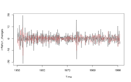
MA processes: changes in inflation tate - II

Inflation_changes: changes in one-month US inflation rate
Plot the series and its sample ACF:

ts.plot(inflation_changes)
acf(inflation_changes, lag.max = 24)

$Today = Mean + Noise + Slope * (Yesterday's Noise)$ $$Y_t = \mu + \epsilon_t + \theta\epsilon_{t-1}$$ $$\epsilon_t ~ WhiteNoise(0, \sigma_{\epsilon}^2)$$

MA_inflation_changes <- arima(inflation_changes, 
                              order = c(0, 0, 1))

print(MA_inflation_changes)

Coefficients:
         ma1  intercept
      -0.7932    0.0010
s.e.   0.0355    0.0281
sigma^2 estimated as 8.882

ma1 = $\hat{\theta}$, intercept = $\hat{\mu}$, sigma^2 = $\hat{\sigma^2_{\epsilon}}$

MA processes: fitted values - I

MA fitted values:

$$\hat{Y_t} = \hat{\mu} +\hat{\theta}\hat{\epsilon_{t-1}}$$

Residuals =

$$\hat{\epsilon_t} = Y_t - \hat{Y_t}$$

ts.plot(inflation_changes)
MA_inflation_changes_fitted <- 
    inflation_changes - residuals(MA_inflation_changes)

points(MA_inflation_changes_fitted, type = "l", 
       col = "red", lty = 2)

Forecasting

1-step ahead forecasts:

predict(MA_inflation_changes)$pred

Jan
1991 4.831632

predict(MA_inflation_changes)$se

Jan
1991 2.980203

Forecasting (cont.)

h-step ahead forecasts:

predict(MA_inflation_changes, n.ahead = 6)$pred

           Jan       Feb       Mar       Apr       May       Jun
1991  4.831632  0.001049  0.001049  0.001049  0.001049  0.001049

predict(MA_inflation_changes, n.ahead = 6)$se

           Jan       Feb       Mar       Apr       May       Jun
1991  2.980203  3.803826  3.803826  3.803826  3.803826  3.803826

Let's practice!

Time Series Analysis in R