Descriptive statistics with R

R For SAS Users

Melinda Higgins, PhD

Research Professor/Senior Biostatistician Emory University

Loading external CSV datasets

Abalone dataset contains 9 measurements:
- length
- diameter
- height
- whole weight
- shucked weight
- shell weight
- viscera weight
- sex (infants, females, males)
- number of rings

abalone picture

For 4177 abalones

Loading external CSV datasets

abalone dataset available in CSV (comma separated value) format
read_csv() function from readr package used to load CSV data

readr hexsticker logo

sas code proc import csv file like r code using read csv function from readr package

sas proc import like read csv function from readr r package

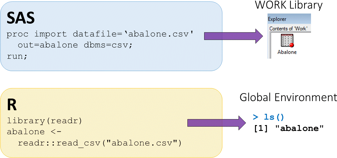
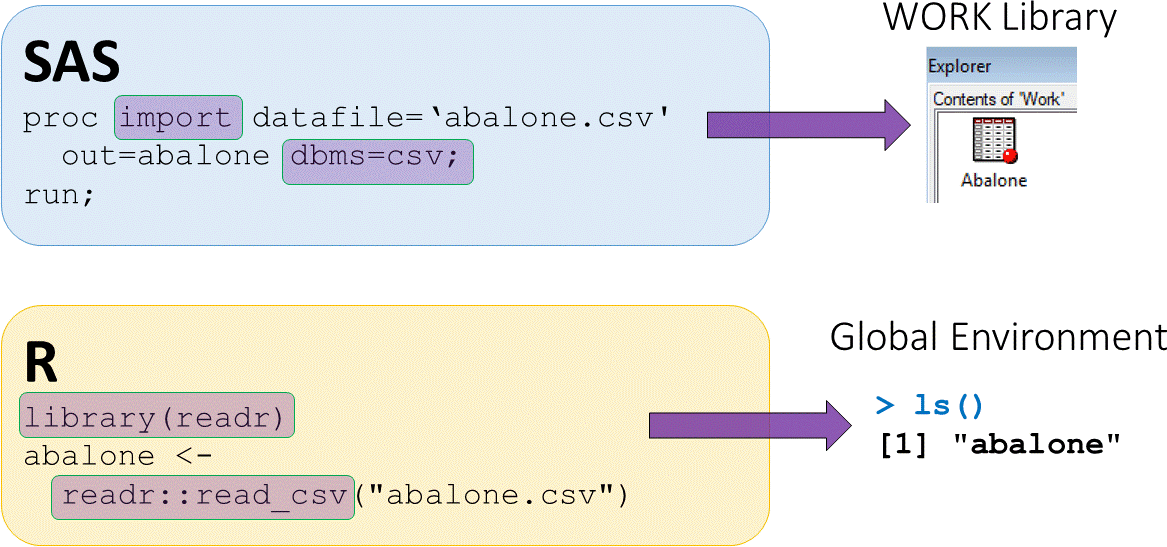
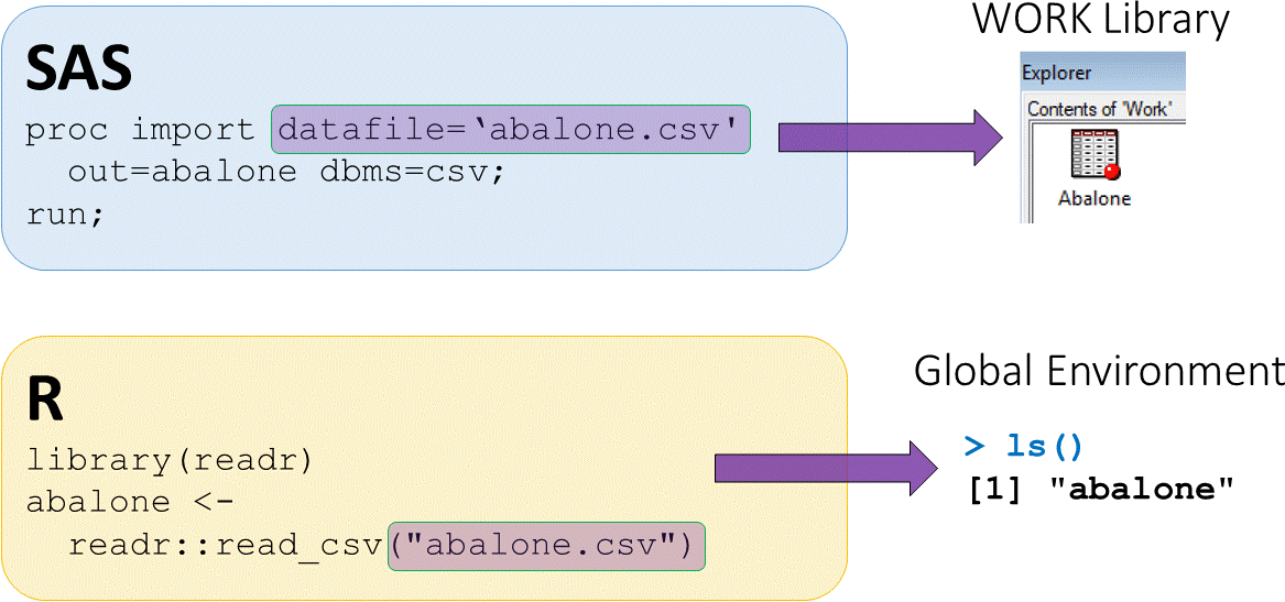
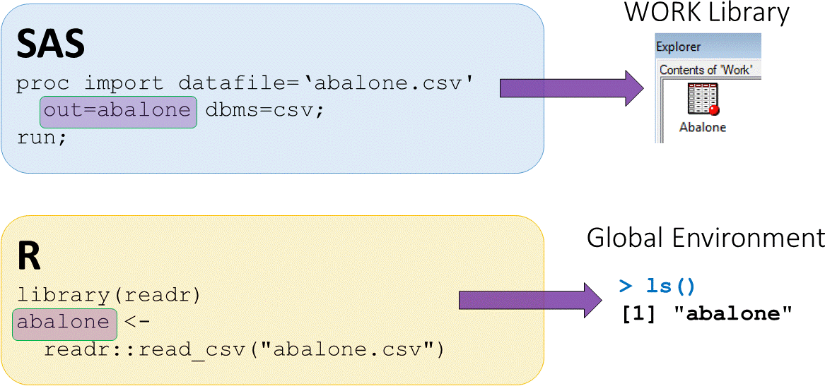
The assign operator <- puts output from readr::read_csv into an object abalone
abalone is now saved in the global environment

sas proc contents like r str structure function

str(abalone)

Classes ‘tbl_df’, ‘tbl’ and 'data.frame':    4177 obs. of  9 variables:
 $ sex          : chr  "M" "M" "F" "M" ...
 $ length       : num  0.455 0.35 0.53 0.44 0.33 0.425 0.53 0.545 ...
 $ diameter     : num  0.365 0.265 0.42 0.365 0.255 0.3 0.415 0.425  ...
 $ height       : num  0.095 0.09 0.135 0.125 0.08 0.095 0.15 0.125 ...
 $ wholeWeight  : num  0.514 0.226 0.677 0.516 0.205 ...
 $ shuckedWeight: num  0.2245 0.0995 0.2565 0.2155 0.0895 ...
 $ visceraWeight: num  0.101 0.0485 0.1415 0.114 0.0395 ...
 $ shellWeight  : num  0.15 0.07 0.21 0.155 0.055 0.12 0.33 0.26 ...
 $ rings        : int  15 7 9 10 7 8 20 16 9 19 ...

sas proc contents like dim dimension and names functions in r

# Display dimensions of abalone dataset
dim(abalone)

4177    9

# Elements or variables in abalone dataset
names(abalone)

"sex"           "length"        "diameter"     "height"        "wholeWeight"   
"shuckedWeight" "visceraWeight" "shellWeight"  "rings"

Dataset contents and variable types

head() and tail() show top and bottom 6 rows respectively by default
Change the number of rows shown by adding a second argument to the function

# Show bottom 7 rows of abalone
tail(abalone, 7)

# A tibble: 7 x 9
  sex   length diameter height wholeWeight shuckedWeight visceraWeight shellWeight rings
  <chr>  <dbl>    <dbl>  <dbl>       <dbl>         <dbl>         <dbl>       <dbl> <dbl>
1 M      0.55     0.43   0.13        0.840         0.316         0.196       0.240    10
2 M      0.56     0.43   0.155       0.868         0.4           0.172       0.229     8
3 F      0.565    0.45   0.165       0.887         0.37          0.239       0.249    11
4 M      0.59     0.44   0.135       0.966         0.439         0.214       0.260    10
5 M      0.6      0.475  0.205       1.18          0.526         0.288       0.308     9
6 F      0.625    0.485  0.15        1.09          0.531         0.261       0.296    10
7 M      0.71     0.555  0.195       1.95          0.946         0.376       0.495    12

Working with data using dplyr approach

dplyr hexsticker logo

In this course, you will use these dplyr functions:

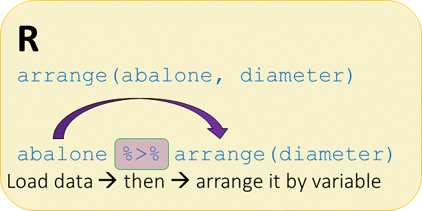
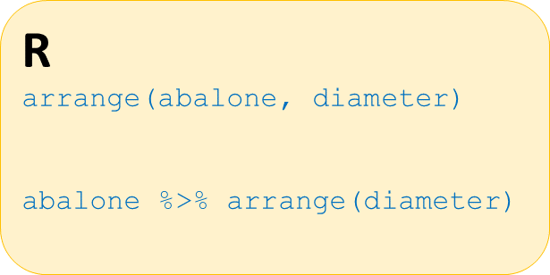
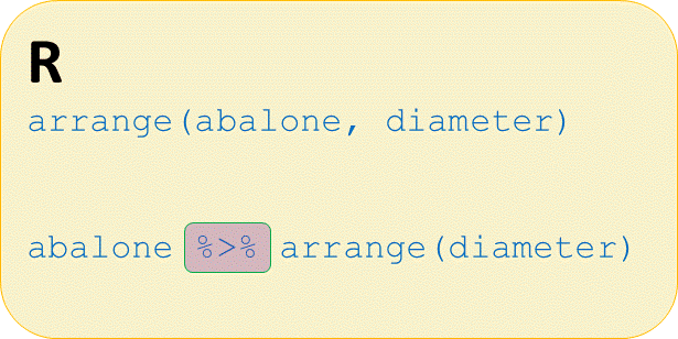
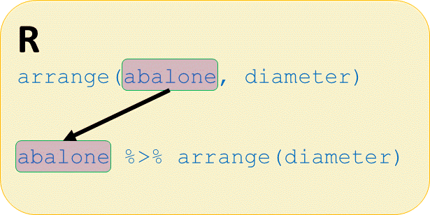
%>% is a pipe operator from the magrittr package included with dplyr
arrange() will sort the data by one or more variables
pull(x) will pull one column x variable out of the dataset
select(x,y,z) will select more than one variable out of the dataset

dplyr arrange function and pipe %>% approach

r arrange function with and without pipe operator

dplyr arrange function and pipe %>% approach

r arrange function with and without pipe operator

dplyr arrange function and pipe %>% approach

r arrange function with and without pipe operator

dplyr arrange function and pipe %>% approach

r arrange function with and without pipe operator

Arrange abalones by diameter

# Arrange abalone dataset by diameter dimension
abalone %>%
  arrange(diameter)

# A tibble: 4,177 x 9
   sex   length diameter height wholeWeight shuckedWeight visceraWeight shellWeight rings
   <chr>  <dbl>    <dbl>  <dbl>       <dbl>         <dbl>         <dbl>       <dbl> <dbl>
 1 I      0.075    0.055  0.01       0.002         0.001         0.0005      0.0015     1
 2 I      0.11     0.09   0.03       0.008         0.0025        0.002       0.003      3
 3 I      0.13     0.095  0.035      0.0105        0.005         0.0065      0.0035     4
 4 I      0.13     0.1    0.03       0.013         0.0045        0.003       0.004      3
 5 I      0.15     0.1    0.025      0.015         0.0045        0.004       0.005      2
 6 I      0.155    0.105  0.05       0.0175        0.005         0.0035      0.005      4
 7 I      0.14     0.105  0.035      0.014         0.0055        0.0025      0.004      3
 8 I      0.17     0.105  0.035      0.034         0.012         0.0085      0.005      4
 9 I      0.14     0.105  0.035      0.0145        0.005         0.0035      0.005      4
10 M      0.155    0.11   0.04       0.0155        0.0065        0.003       0.005      3

Extract one variable from abalone

Let's extract shuckedWeight from abalone using pull() from dplyr

# Pull out shuckedWeight variable from abalone
abalone %>%
  pull(shuckedWeight)

   [1] 0.2245 0.0995 0.2565 0.2155 0.0895 0.1410 0.2370 0.2940 0.2165 0.3145 0.1940 0.1675
  [13] 0.2175 0.2725 0.1675 0.2580 0.0950 0.1880 0.0970 0.1705 0.0955 0.0800 0.4275 0.3180
  [25] 0.5130 0.3825 0.3945 0.3560 0.3940 0.3930 0.3935 0.6055 0.5515 0.8150 0.6330 0.2270
  [37] 0.5305 0.2370 0.3810 0.1340 0.1865 0.3620 0.0315 0.0255 0.0175 0.0875 0.2930 0.1775
  [49] 0.0755 0.3545 0.2385 0.1335 0.2595 0.2105 0.1730 0.2565 0.1920 0.2765 0.0420 0.2460
  [61] 0.1800 0.3050 0.3020 0.1705 0.2340 0.2340 0.3540 0.4160 0.2135 0.0630 0.2640 0.1405
  [73] 0.4800 0.4740 0.4810 0.4425 0.3625 0.3630 0.2820 0.4695 0.3845 0.5105 0.3960 0.4080
  [85] 0.3800 0.3390 0.4825 0.3305 0.2205 0.3135 0.3410 0.3070 0.4015 0.5070 0.5880 0.5755
  [97] 0.2690 0.2140 0.2010 0.2775 0.1050 0.3280 0.3160 0.3105 0.4975 0.2910 0.2935 0.2610
...remaining output removed...

Compute mean and median shucked weight

# Compute mean shuckedWeight
abalone %>%
  pull(shuckedWeight) %>%
  mean()

0.3593675

# Compute median shuckedWeight
abalone %>%
  pull(shuckedWeight) %>%
  median()

0.336

Select two variables from abalone

# Select two variables length and height
abalone %>%
  select(length, height)

# A tibble: 4,177 x 2
   length height
    <dbl>  <dbl>
 1  0.455  0.095
 2  0.35   0.09
 3  0.53   0.135
 4  0.44   0.125
 5  0.33   0.08
 6  0.425  0.095
 7  0.53   0.15
 8  0.545  0.125
# ... with 4,169 more rows

Get summary statistics of length and height

summary() outputs min, max, mean, median and 25th and 75th quartiles

# Get summary stats of length and height
abalone %>%
  select(length, height) %>%
  summary()

     length          height      
 Min.   :0.075   Min.   :0.0000  
 1st Qu.:0.450   1st Qu.:0.1150  
 Median :0.545   Median :0.1400  
 Mean   :0.524   Mean   :0.1395  
 3rd Qu.:0.615   3rd Qu.:0.1650  
 Max.   :0.815   Max.   :1.1300

Let's go find out about abalones

R For SAS Users