Data quality and cleaning

R For SAS Users

Melinda Higgins, PhD

Research Professor/Senior Biostatistician Emory University

Check distributions

# Continue with davismod
davismod %>%
  head(5)

  sex weight height repwt repht      bmi diffht difflow          bmicat
1   M     77    182    77   180 23.24598     -2   FALSE 1. underwt/norm
2   F     58    161    51   159 22.37568     -2   FALSE 1. underwt/norm
3   F     53    161    54   158 20.44674     -3    TRUE 1. underwt/norm
4   M     68    177    70   175 21.70513     -2   FALSE 1. underwt/norm
5   F     59    157    59   155 23.93606     -2   FALSE 1. underwt/norm

Check distributions

# Get summary statistics for bmi, check min, max, median
davismod %>%
  pull(bmi) %>%
  summary()

   Min. 1st Qu.  Median    Mean 3rd Qu.    Max.
  15.82   20.23   21.84   24.70   23.94  510.93

Notice that Max. > 500

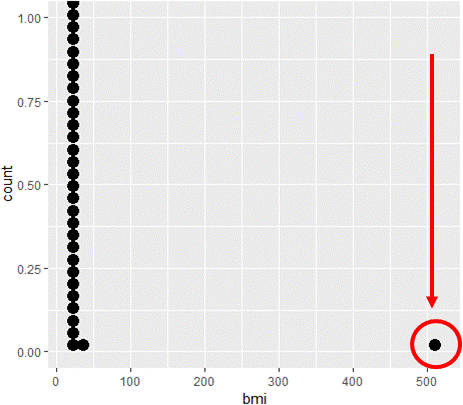
Visualize distributions

# Make bmi dotplot with geom_dotplot()
ggplot(davismod, aes(bmi)) +
  geom_dotplot()

dotplot of bmi

Find the outliers

# Sort data use arrange(), view last 6 rows with tail()
davismod %>%
  arrange(bmi) %>%
  tail()

    sex weight height repwt repht       bmi diffht difflow    bmicat
195   M     89    173    86   173  29.73704      0   FALSE 2. overwt
196   M    102    185   107   185  29.80278      0   FALSE 2. overwt
197   M    103    185   101   182  30.09496     -3    TRUE  3. obese
198   M    101    183   100   180  30.15916     -3    TRUE  3. obese
199   M    119    180   124   178  36.72840     -2   FALSE  3. obese
200   F    166     57    56   163 510.92644    106   FALSE  3. obese

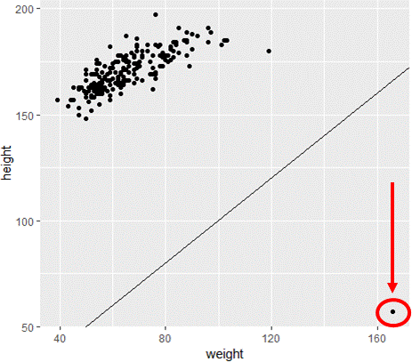
Visualize assumption that weight <= height

# Scatterplot with y=x reference line
ggplot(davismod,
       aes(weight, height)) +
  geom_point() +
  geom_abline(intercept=0, slope=1)

scatterplot height by weight for davismod

Filter out cases with errors

# Use filter() from dplyr, keep cases for bmi < 100
daviskeep <- davismod %>%
  filter(bmi < 100)

# View last 6 rows
daviskeep %>%
  arrange(bmi) %>%
  tail()

    sex weight height repwt repht      bmi diffht difflow    bmicat
194   F     75    162    75   158 28.57796     -4    TRUE 2. overwt
195   M     89    173    86   173 29.73704      0   FALSE 2. overwt
196   M    102    185   107   185 29.80278      0   FALSE 2. overwt
197   M    103    185   101   182 30.09496     -3    TRUE  3. obese
198   M    101    183   100   180 30.15916     -3    TRUE  3. obese
199   M    119    180   124   178 36.72840     -2   FALSE  3. obese

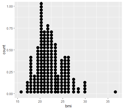
Visualize corrected bmi

# Make dotplot of bmi
ggplot(daviskeep, aes(bmi)) +
  geom_dotplot()

dotplot of bmi from daviskeep

Final cleanup of abalone dataset

Check the assumptions of the abalone dataset
Remove cases that violate assumptions
Finalize dataset for analysis and models

ASSUMPTIONS:

All measurements should be > 0
length is the longest shell dimension
height and diameter < length
wholeWeight is the total weight
Other weights < wholeWeight

abalone shell picture

Let's explore and clean up the abalone dataset

R For SAS Users