ANOVA and linear models

R For SAS Users

Melinda Higgins, PhD

Research Professor/Senior Biostatistician Emory University

Note on missing values

# Stats by bmicat - descriptives for ANOVA
daviskeep %>%
  group_by(bmicat) %>%
  select(diffht, bmicat) %>%
  summarise(across(everything(),
                   list(mean = ~mean(.x),
                        sd = ~sd(.x),
                        var = ~var(.x))),
            N = n())

# A tibble: 3 × 5
  bmicat          diffht_mean diffht_sd diffht_var     N
  <chr>                 <dbl>     <dbl>      <dbl> <int>
1 1. underwt/norm       NA       NA         NA       161
2 2. overwt             NA       NA         NA        35
3 3. obese              -2.67     0.577      0.333     3

Note on missing values

# Stats by bmicat - descriptives for ANOVA
daviskeep %>%
  group_by(bmicat) %>%
  select(diffht, bmicat) %>%
  summarise(across(everything(),
                   list(mean = ~mean(.x, na.rm = TRUE),
                        sd = ~sd(.x, na.rm = TRUE),
                        var = ~var(.x, na.rm = TRUE))),
            N = n())

# A tibble: 3 × 5
  bmicat          diffht_mean diffht_sd diffht_var     N
  <chr>                 <dbl>     <dbl>      <dbl> <int>
1 1. underwt/norm       -2.12     2.14       4.56    161
2 2. overwt             -1.78     1.91       3.66     35
3 3. obese              -2.67     0.577      0.333     3

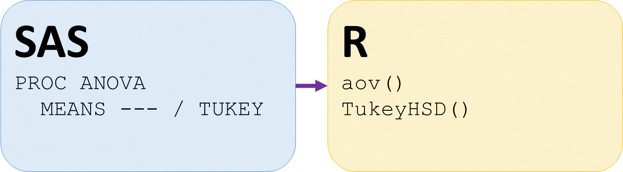
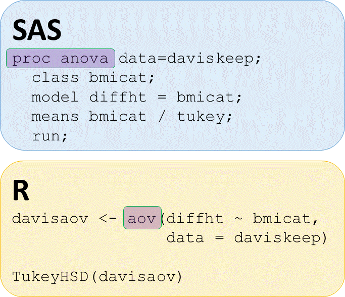
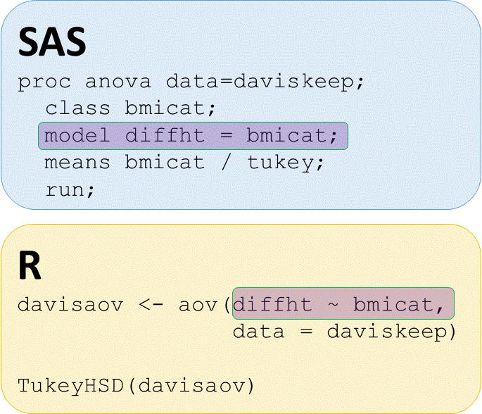
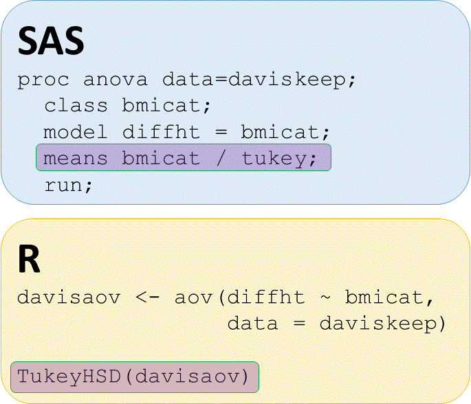
Analysis of Variance (ANOVA) SAS and R

SAS PROC ANOVA and R aov and TukeyHSD functions

SAS PROC ANOVA and R aov function

SAS PROC ANOVA and R aov function model statement

SAS PROC ANOVA and R aov function tukey comparisons

Analysis of Variance (ANOVA)

# Perform ANOVA of diffht by bmicat, save output as davisaov
davisaov <- aov(diffht ~ bmicat, data = daviskeep)

# Show summary of davisaov
summary(davisaov)

             Df Sum Sq Mean Sq F value Pr(>F)
bmicat        2    4.1   2.070   0.475  0.623
Residuals   179  779.9   4.357               
17 observations deleted due to missingness

Post hoc pairwise tests

# Perform TukeyHSD posthoc pairwise tests on abaov
TukeyHSD(davisaov)

  Tukey multiple comparisons of means
    95% family-wise confidence level

Fit: aov(formula = diffht ~ bmicat, data = daviskeep)

$bmicat
                                diff        lwr      upr     p adj
2. overwt-1. underwt/norm  0.3411990 -0.6211376 1.303536 0.6799698
3. obese-1. underwt/norm  -0.5442177 -3.4213543 2.332919 0.8957761
3. obese-2. overwt        -0.8854167 -3.8641564 2.093323 0.7623194

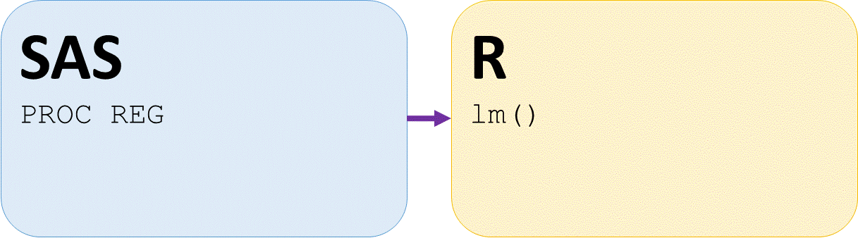
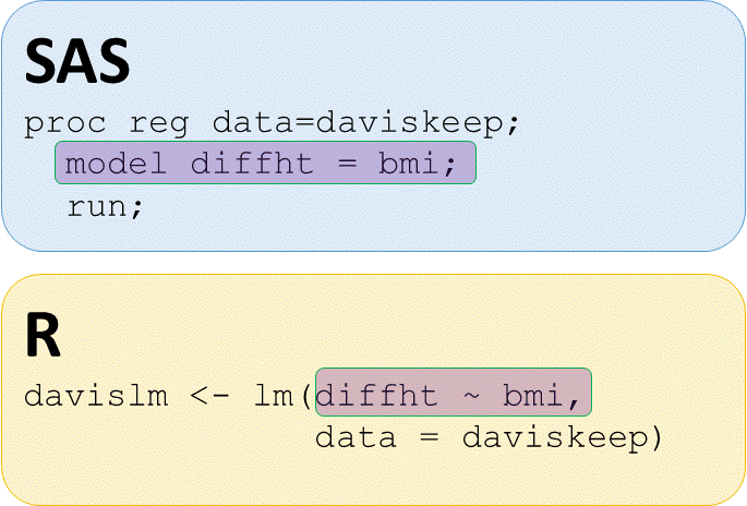
Linear regression SAS and R

SAS PROC REG and R lm function

SAS PROC REG and R lm function model statement

Simple linear regression

# Run lm() of diffht by bmi
davislm <- lm(diffht ~ bmi,
              data = daviskeep)
davislm

# Display elements in davislm
names(davislm)

Call:
lm(formula = diffht ~ bmi,
   data = daviskeep)

Coefficients:
(Intercept)          bmi  
   -2.60878      0.02404

 [1] "coefficients"  "residuals"    
 [3] "effects"       "rank"         
 [5] "fitted.values" "assign"       
 [7] "qr"            "df.residual"  
 [9] "na.action"     "xlevels"      
[11] "call"          "terms"        
[13] "model"

Simple linear regression

# Display coefficients element
davislm$coefficients

(Intercept)         bmi
-2.60877657  0.02403939

# Display the slope coefficient 2
davislm$coefficients[2]

       bmi
0.02403939

summary(davislm)

Call:
lm(formula = diffht ~ bmi, data = daviskeep)

Residuals:
    Min      1Q  Median      3Q     Max
-7.8607 -0.9944 -0.0048  1.1271  8.1627

Coefficients:
            Estimate Std. Error t value Pr(>|t|)  
(Intercept) -2.60878    1.15718  -2.254   0.0254 *
bmi          0.02404    0.05130   0.469   0.6399  

Signif. codes:  0 ‘***’ 0.001 ‘**’ 0.01 ‘*’ 0.05 ‘.’ 0.1 ‘ ’ 1

Residual standard error: 2.086 on 180 degrees of freedom
  (17 observations deleted due to missingness)
Multiple R-squared:  0.001218,    Adjusted R-squared:  -0.004331
F-statistic: 0.2196 on 1 and 180 DF,  p-value: 0.6399

Summary of linear regression model

# Save summary() output of lmshucked, see element names
smrydavislm <- summary(davislm)
names(smrydavislm)

 [1] "call"          "terms"         "residuals"     "coefficients"
 [5] "aliased"       "sigma"         "df"            "r.squared"    
 [9] "adj.r.squared" "fstatistic"    "cov.unscaled"  "na.action"

Summary of linear regression model

# Display r.squared from smrydavislm
smrydavislm$r.squared

[1] 0.00121824

# Display coefficients from smrydavislm
smrydavislm$coefficients

               Estimate Std. Error    t value   Pr(>|t|)
(Intercept) -2.60877657 1.15717685 -2.2544320 0.02537425
bmi          0.02403939 0.05130456  0.4685624 0.63994943

Let's go fit and explore models for abalones!

R For SAS Users