Commuting Patterns

Analyzing US Census Data in Python

Lee Hachadoorian

Asst. Professor of Instruction, Temple University

Commuting Tables

Commuting Subjects

Means of transportation (car, public transit, etc.)
Travel time
Time leaving for/arriving at work

Commuting Geographies

Residence: where people sleep
Workplace: where people work; can use to determine workforce population for county, tract, etc.

Congestion Pricing in New York City

Currently being debated in NYC (early 2019)
Previous attempt failed (2007)
Concerns over cost for low- and middle-income households

Overhead photograph of cars and taxicabs on a street in New York City.

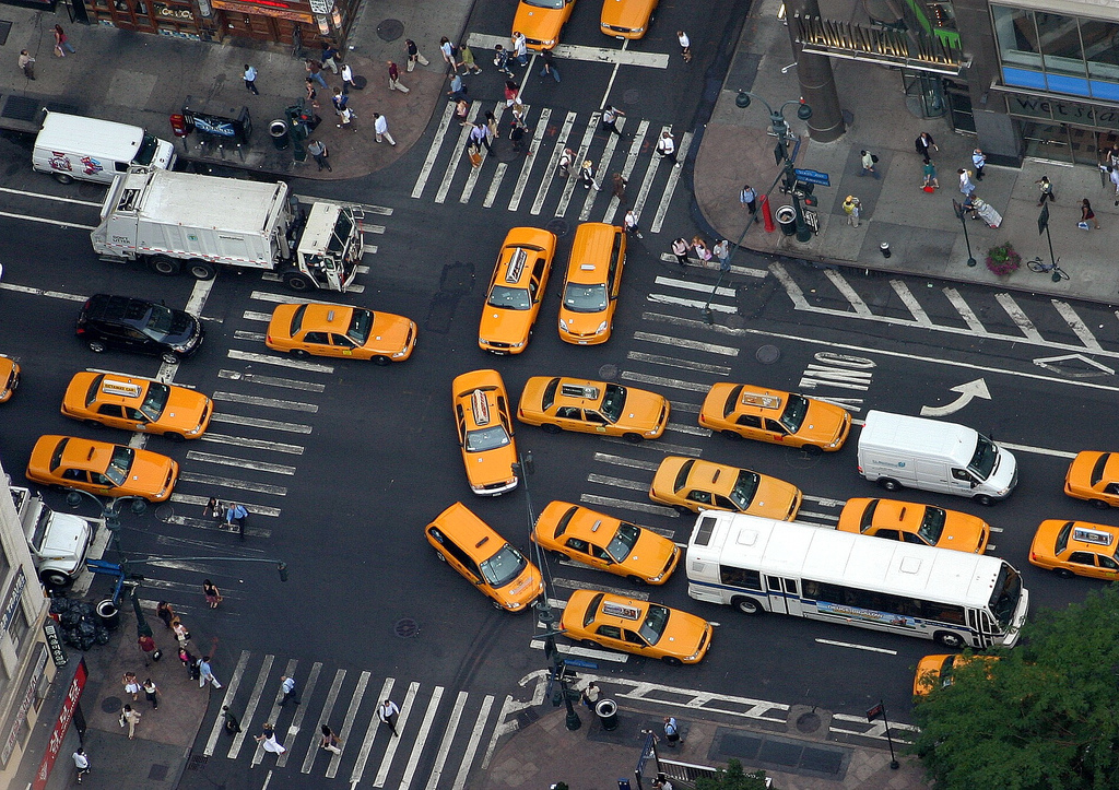
¹ Photo by Brian Jeffery Beggerly (CC BY 2.0)

Table B08519: Means Of Transportation To Work By Workers' Earnings In The Past 12 Months (In 2017 Inflation-Adjusted Dollars) For Workplace Geography

Total
    $1 to $9,999 or loss
    $10,000 to $14,999
    $15,000 to $24,999
    $25,000 to $34,999
    $35,000 to $49,999
    $50,000 to $64,999
    $65,000 to $74,999
    $75,000 or more
Car truck or van - drove alone
    <repeat income categories>
Car truck or van - carpooled
    <repeat income categories>
Public transportation (excluding taxicab)
    <repeat income categories>
etc...

API Response

print(r.json())

[['B08519_011E', 'B08519_012E', 'B08519_013E', 'B08519_014E', 'B08519_015E',
  'B08519_016E', 'B08519_017E', 'B08519_018E', 'B08519_020E', 'B08519_021E', 
  ... 
  'B08519_061E', 'B08519_062E', 'B08519_063E', 'state', 'county'], 
 ['10927', '9172', '19659', '22110', '32287', 
  '32977', '15693', '106972', '3663', '2518', 
  ...
  '7457', '2664', '20684', '36', '061']]

Reshaping the Data

# Read data row into list
data_row = r.json()[1][:-2]

# Break data row into list of lists
iter_len = 8
data = [data_row[i:i+iter_len] for i in range(0, len(data_row), iter_len)]

print(data)

[['10927', '9172', '19659', '22110', '32287', '32977', '15693', '106972'], 
['3663', '2518', '5484', '5625', '8028', '7990', '3369', '22958'], 
['139358', '97178', '200514', '184510', '255491', '240973', '116673', '700808'], 
['16743', '9117', '15900', '13710', '17442', '20206', '10370', '85879'], ...]

Constructing the DataFrame

# Define row names and column names
modes = ["drove_alone", "carpooled", "public", "walked", "taxi", 
         "worked_at_home"]

incomes = ["0k", "10k", "15k", "25k", "35k", "50k", "65k", "75k"]

# Create DataFrame
manhattan = pd.DataFrame(data=data, index=modes, columns=incomes)
manhattan = manhattan.astype(int)

Constructing the DataFrame

print(manhattan)

                    0k    10k     15k   ...       50k     65k     75k
drove_alone      10716   8965   19294   ...     31502   15519  104078
carpooled         3740   2451    5852   ...      7994    3438   22625
public          140957  99474  197241   ...    235158  111959  654800
walked           16795   9045   15451   ...     20704   10663   83681
taxi              3201   2209    4515   ...      6551    3029   35572
worked_at_home    6854   3885    5489   ...      7776    2809   19598

[6 rows x 8 columns]

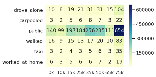
Constructing the Heatmap

# Create heatmap of commuters by mode by income
sns.heatmap(manhattan, annot=manhattan // 1000, fmt="d", cmap="YlGnBu")

A heatmap showing rows of commute modes and columns of income categories colored by the number of commuters in each cell. The row of public transit commuters is darker, and the cell of public transit commuters with incomes over $75,000 is the darkest.

Let's practice!

Analyzing US Census Data in Python