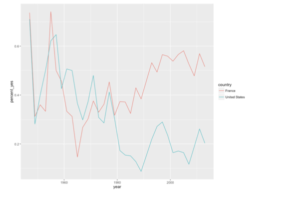
Visualizing by country

Case Study: Exploratory Data Analysis in R

Dave Robinson

Chief Data Scientist, DataCamp

Examining by country and year

Summarizing by country and year

by_year_country <- votes_processed %>%
  group_by(year, country) %>%
  summarize(total = n(),
              percent_yes = mean(vote == 1))
by_year_country

# A tibble: 4,744 × 4
# Groups:   year [34]
   year     country total percent_yes
  <dbl>       <chr> <int>       <dbl>
1  1947 Afghanistan    34   0.3823529
2  1947   Argentina    38   0.5789474
3  1947   Australia    38   0.5526316
4  1947     Belarus    38   0.5000000
5  1947     Belgium    38   0.6052632
# ... with 4,739 more rows

Filtering for one country

by_year_country %>%
  filter(country == "United States")

# A tibble: 34 × 4
    year       country total percent_yes
   <dbl>         <chr> <int>       <dbl>
1   1947 United States    38   0.7105263
2   1949 United States    64   0.2812500
3   1951 United States    25   0.4000000
4   1953 United States    26   0.5000000
5   1955 United States    37   0.6216216
6   1957 United States    34   0.6470588
7   1959 United States    54   0.4259259
8   1961 United States    75   0.5066667
9   1963 United States    32   0.5000000
10  1965 United States    41   0.3658537
# ... with 24 more rows

2-2_v2.011.png

The %in% operator

c("A", "B", "C", "D", "E") %in% c("B", "E")

FALSE  TRUE FALSE FALSE  TRUE

Filtering for multiple countries

us_france <- by_year_country %>%
  filter(country %in% c("United States", "France"))
us_france

# A tibble: 68 × 4
    year       country total percent_yes
   <dbl>         <chr> <int>       <dbl>
1   1947        France    38   0.7368421
2   1947 United States    38   0.7105263
3   1949        France    64   0.3125000
4   1949 United States    64   0.2812500
5   1951        France    25   0.3600000
6   1951 United States    25   0.4000000
7   1953        France    18   0.3333333
8   1953 United States    26   0.5000000
9   1955        France    27   0.7407407
10  1955 United States    37   0.6216216
# ... with 58 more rows

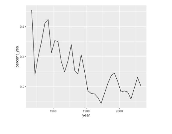
Visualizing vote trends by country

# A tibble: 68 × 4
    year       country total percent_yes
   <dbl>         <chr> <int>       <dbl>
1   1947        France    38   0.7368421
2   1947 United States    38   0.7105263
3   1949        France    64   0.3125000
4   1949 United States    64   0.2812500
5   1951        France    25   0.3600000
6   1951 United States    25   0.4000000
7   1953        France    18   0.3333333
8   1953 United States    26   0.5000000
9   1955        France    27   0.7407407
10  1955 United States    37   0.6216216
# ... with 58 more rows

ggplot(us_france, aes(x = year, y = percent_yes,
                      color = country)) +
  geom_line()

2-2_v2.022.png

Let's practice!

Case Study: Exploratory Data Analysis in R