Nesting for multiple models
Case Study: Exploratory Data Analysis in R

Dave Robinson
Chief Data Scientist, DataCamp
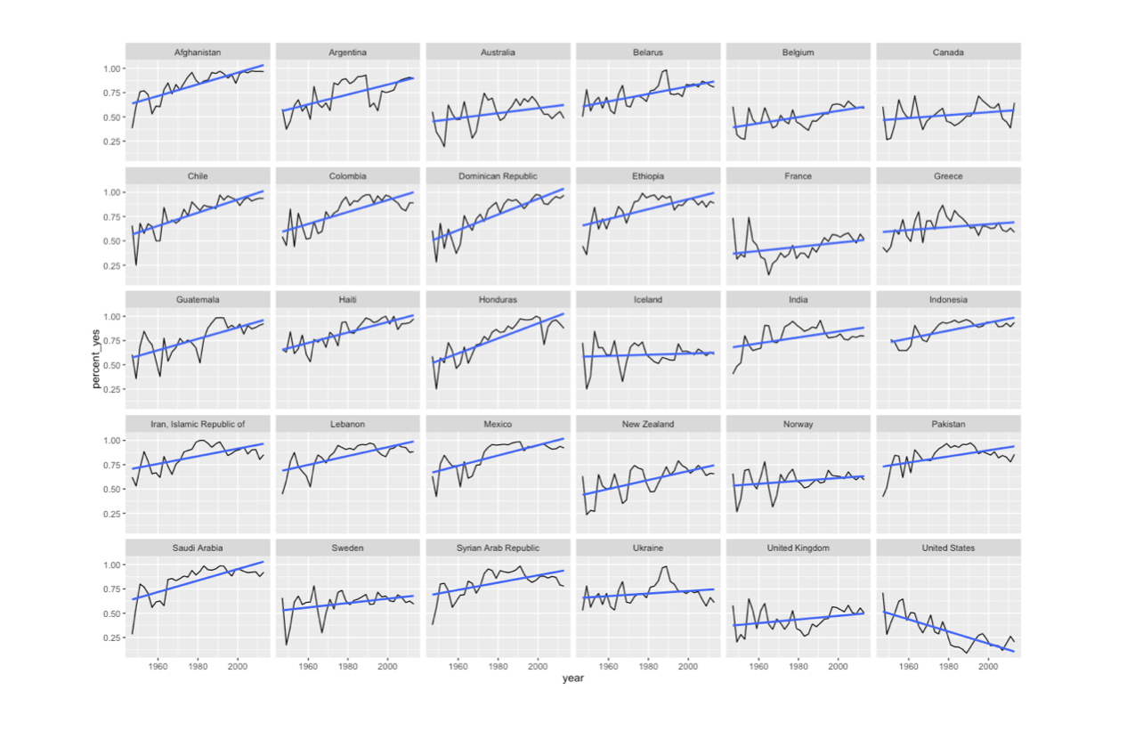
One model for each country
Start with one row per country
by_year_country
# A tibble: 4,744 × 4
    year                         country total percent_yes
   <dbl>                           <chr> <int>       <dbl>
1   1947                     Afghanistan    34   0.3823529
2   1947                       Argentina    38   0.5789474
3   1947                       Australia    38   0.5526316
4   1947                         Belarus    38   0.5000000
5   1947                         Belgium    38   0.6052632
6   1947 Bolivia, Plurinational State of    37   0.5945946
7   1947                          Brazil    38   0.6578947
8   1947                          Canada    38   0.6052632
9   1947                           Chile    38   0.6578947
10  1947                        Colombia    35   0.5428571
# ... with 4,734 more rows
nest() turns it into one row per country
library(tidyr)
by_year_country %>%
  nest(-country)
# A tibble: 200 × 2
                           country              data
                             <chr>            <list>
1                      Afghanistan <tibble [34 × 3]>
2                        Argentina <tibble [34 × 3]>
3                        Australia <tibble [34 × 3]>
4                          Belarus <tibble [34 × 3]>
5                          Belgium <tibble [34 × 3]>
6  Bolivia, Plurinational State of <tibble [34 × 3]>
7                           Brazil <tibble [34 × 3]>
8                           Canada <tibble [34 × 3]>
9                            Chile <tibble [34 × 3]>
10                        Colombia <tibble [34 × 3]>
# ... with 190 more rows
-countrymeans “nest all except country”
- “nested” year, total, percent_yes data for just Afghanistan
# A tibble: 34 × 3
     year total percent_yes
    <dbl> <int>       <dbl>
1    1947    34   0.3823529
2    1949    51   0.6078431
3    1951    25   0.7600000
4    1953    26   0.7629308
5    1955    37   0.7297297
6    1957    34   0.5294118
7    1959    54   0.6111111
8    1961    76   0.6052632
9    1963    32   0.7812500
10   1965    40   0.8500000

# ... with 24 more rows
unnest() does the opposite
by_year_country %>%
  nest(-country) %>%
  unnest(data)
# A tibble: 4,744 × 4
    year total percent_yes        country
   <dbl> <int>       <dbl>          <chr>
1   1947    34   0.3823529    Afghanistan
2   1947    38   0.5789474      Argentina
3   1947    38   0.5789474 United Kingdom
4   1947    38   0.5526316      Australia
5   1947    38   0.5000000        Belarus
6   1947    38   0.5000000          Egypt
7   1947    38   0.5000000   South Africa
8   1947    38   0.5000000     Yugoslavia
9   1947    38   0.6052632        Belgium
10  1947    38   0.6052632         Canada
Let's practice!
Case Study: Exploratory Data Analysis in R

