Introduction to Text Analysis in R
Maham Faisal Khan
Senior Data Science Content Developer
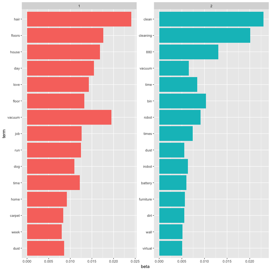
lda_topics <- LDA(
  dtm_review,
  k = 2,
  method = "Gibbs",
  control = list(seed = 42)
) %>%
  tidy(matrix = "beta")

word_probs <- lda_topics %>%
  group_by(topic) %>%
  slice_max(beta, n = 15) %>%
  ungroup() %>%
  mutate(term2 = fct_reorder(term, beta))
lda_topics <- LDA( dtm_review, k = 2, method = "Gibbs", control = list(seed = 42) ) %>% tidy(matrix = "beta")
word_probs <- lda_topics %>% group_by(topic) %>% slice_max(beta, n = 15) %>% ungroup() %>% mutate(term2 = fct_reorder(term, beta))
ggplot(
  word_probs,
  aes(
    term2,
    beta,
    fill = as.factor(topic)
  )
) +
  geom_col(show.legend = FALSE) +
  facet_wrap(~ topic, scales = "free") +
  coord_flip()
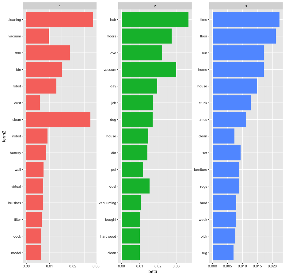
lda_topics2 <- LDA(
  dtm_review,
  k = 3,
  method = "Gibbs",
  control = list(seed = 42)
) %>%
  tidy(matrix = "beta")

word_probs2 <- lda_topics2 %>%
  group_by(topic) %>%
  slice_max(beta, n = 15) %>%
  ungroup() %>%
  mutate(term2 = fct_reorder(term, beta))
lda_topics2 <- LDA( dtm_review, k = 3, method = "Gibbs", control = list(seed = 42) ) %>% tidy(matrix = "beta")
word_probs2 <- lda_topics2 %>% group_by(topic) %>% slice_max(beta, n = 15) %>% ungroup() %>% mutate(term2 = fct_reorder(term, beta))
ggplot(
  word_probs2,
  aes(
    term2,
    beta,
    fill = as.factor(topic)
  )
) +
  geom_col(show.legend = FALSE) +
  facet_wrap(~ topic, scales = "free") +
  coord_flip()