Hiding unused cells

Loan Amortization in Google Sheets

Brent Allen

Instructor

Easier to subtract than add
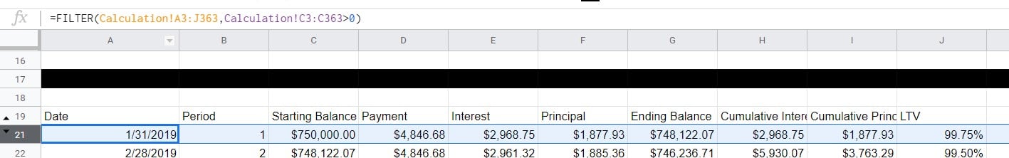
  • Create a schedule with more periods than you think you will need.
  • Bi-weekly X 30 years = 780 periods!
  • Visualizations will continue to show incomplete periods.
  • Schedule will show N/A values where formulas can't be calculated properly.

Visualization with no hidden periods

Loan Amortization in Google Sheets

Methods to hide unused cells

Create filtered table

  • Uses FILTER() formula to create a second table which is filtered for required periods.
  • Simple formula, but can't do advanced calculations.

Hide with logical functions

  • Uses IFS() formula to hide cells which are past the final amortization period.
  • More complex formula, but offers more flexibility.
Loan Amortization in Google Sheets

The FILTER formula

FILTER() _ hides rows or columns from a table based on specified conditions._

  • Move the existing table to the right side or another sheet.
  • Refer to the entire data table in the FILTER() formula.

=FILTER(original table, opening balance column > 0)

Example of the FILTER function

Loan Amortization in Google Sheets

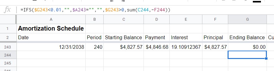
Hiding cells with IFS

2 reasons to hide a cell using an IFS() formula

  • Closing balance in prior cell is zero.

=IFS($G243<0.01,""

  • Prior row is blank.

,$A243="","",

If neither condition is met, use the formula for the column
,$G243>0,sum(C244,-F244))

IFS formula for hiding cells

Loan Amortization in Google Sheets

Tips with IFS formula

  • The same column can be used to check for blanks in all formulas.

=IFS($G243<0.01,"",$A243="","",$G243>0,SUM(C244,-F244))

=IFS($G243<0.01,"",$A243="","",$G243>0,E244+H243)

  • Replace values with ROW() formula for period.

=IFS($G243<0.01,"",$A243="","",$G243>0,ROW()-3)

  • Copy values from period 1 to bottom.
Loan Amortization in Google Sheets

Time to fix some schedules!

Loan Amortization in Google Sheets

Preparing Video For Download...