Using the randomization distribution
Foundations of Inference in R

Jo Hardin
Instructor
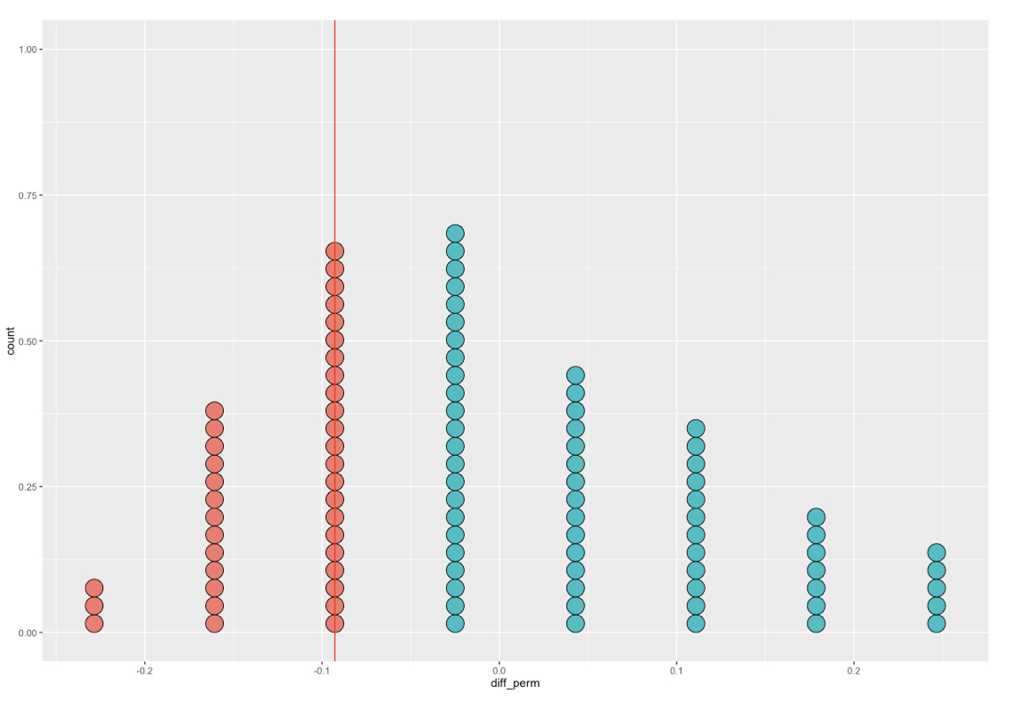
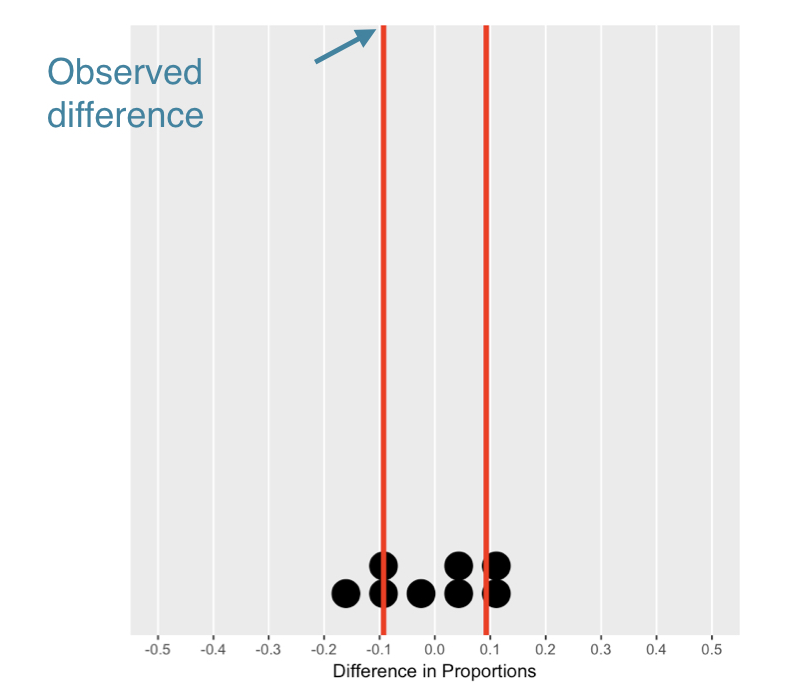
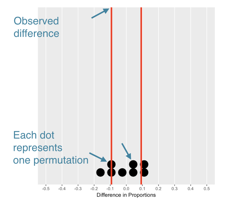
Understanding the null distribution
Understanding the null distribution
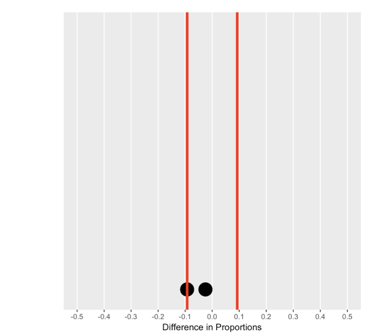
Understanding the null distribution
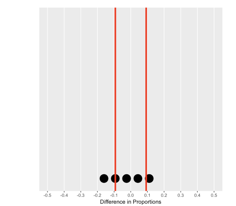
Understanding the null distribution
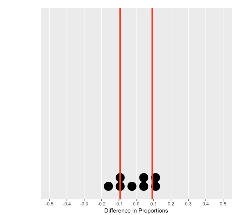
Understanding the null distribution
Significance