AR and MA models
ARIMA Models in R

David Stoffer
Professor of Statistics at the University of Pittsburgh
AR and MA Models
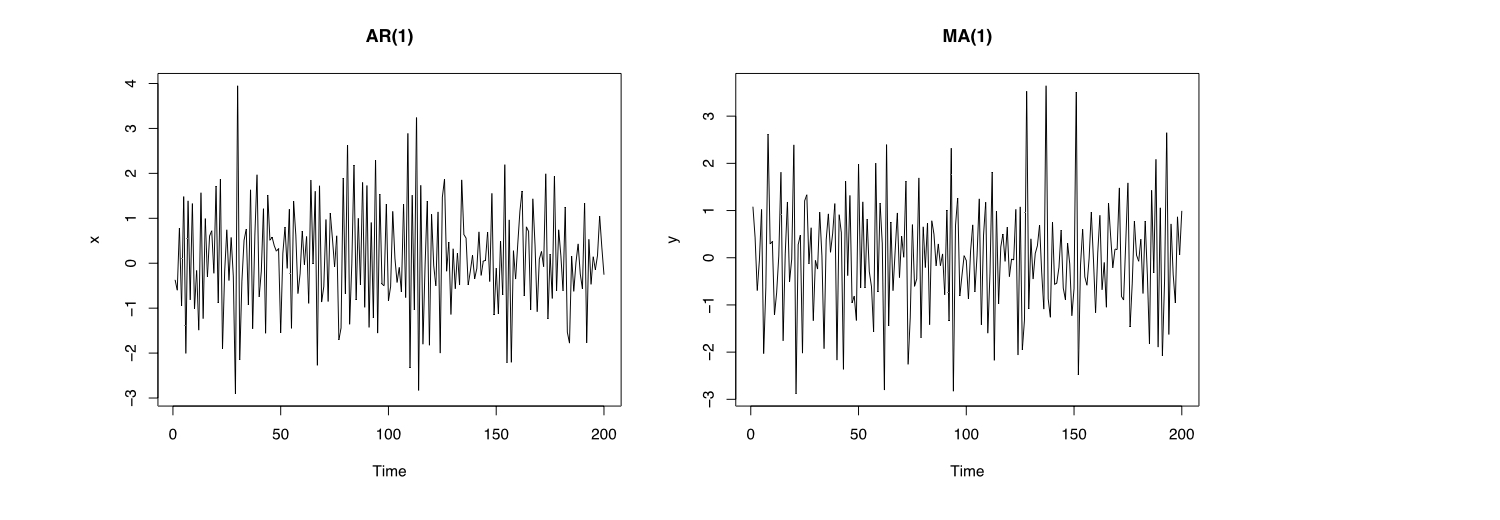
x <- arima.sim(list(order = c(1, 0, 0), ar = -.7), n = 200)
y <- arima.sim(list(order = c(0, 0, 1), ma = -.7), n = 200)
par(mfrow = c(1, 2))
plot(x, main = "AR(1)")
plot(y, main = "MA(1)")
ACF and PACF
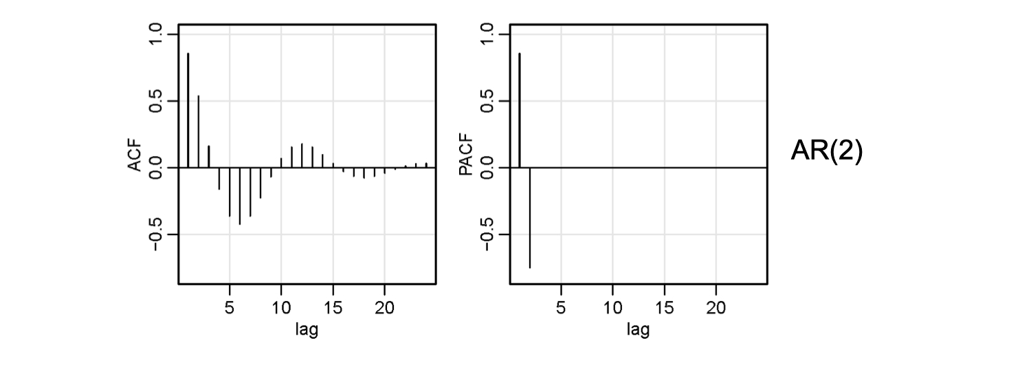
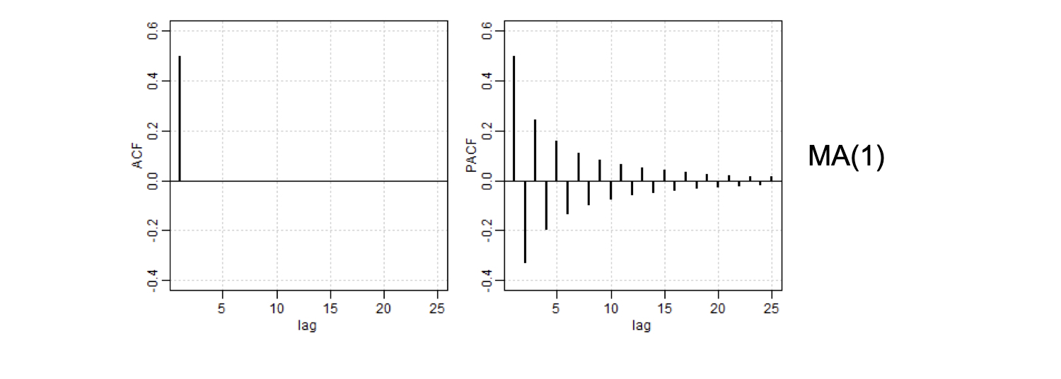
| AR(p) | MA(q) | ARMA(p, q) | |
|---|---|---|---|
| ACF | Tails off | Cuts off lag q | Tails off |
| PACF | Cuts off lag p | Tails off | Tails off |
ACF and PACF
| AR(p) | MA(q) | ARMA(p, q) | |
|---|---|---|---|
| ACF | Tails off | Cuts off lag q | Tails off |
| PACF | Cuts off lag p | Tails off | Tails off |
Estimation
- Estimation for time series is similar to using least squares for regression
- Estimates are obtained numerically using ideas of Gauss and Newton