Modern portfolio theory

Introduction to Portfolio Analysis in Python

Charlotte Werger

Data Scientist

Creating optimal portfolios

Icon for investment strategy

What is Portfolio Optimization?

Meet Harry Markowitz

Harry Markowitz

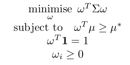
The optimization problem: finding optimal weights

$$ Markowitz' optimization problem

In words:

Minimize the portfolio variance, subject to:
The expected mean return is at least some target return
The weights sum up to 100%
At least some weights are positive

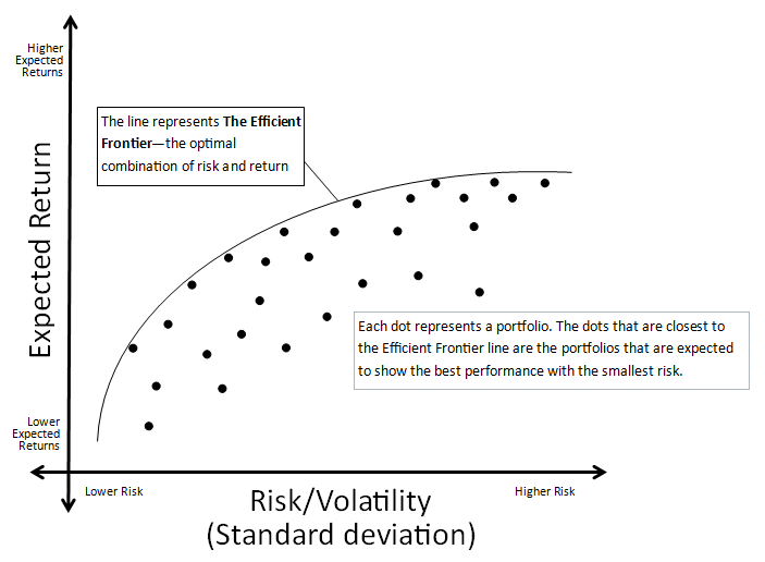
Varying target returns leads to the Efficient Frontier

Graph of the efficient frontier

PyPortfolioOpt for portfolio optimization

from pypfopt.efficient_frontier import EfficientFrontier
from pypfopt import risk_models
from pypfopt import expected_returns

df=pd.read_csv('portfolio.csv')
df.head(2)
                XOM        RRC        BBY         MA        PFE       
date
2010-01-04  54.068794  51.300568  32.524055  22.062426  13.940202 
2010-01-05  54.279907  51.993038  33.349487  21.997149  13.741367

# Calculate expected annualized returns and sample covariance
mu = expected_returns.mean_historical_return(df)
Sigma = risk_models.sample_cov(df)

Get the Efficient Frontier and portfolio weights

# Calculate expected annualized returns and risk
mu = expected_returns.mean_historical_return(df)
Sigma = risk_models.sample_cov(df)

# Obtain the EfficientFrontier
ef = EfficientFrontier(mu, Sigma)

# Select a chosen optimal portfolio
ef.max_sharpe()

Different optimizations

# Select the maximum Sharpe portfolio
ef.max_sharpe()

# Select an optimal return for a target risk 
ef.efficient_risk(2.3)

# Select a minimal risk for a target return
ef.efficient_return(1.5)

Calculate portfolio risk and performance

# Obtain the performance numbers
ef.portfolio_performance(verbose=True, risk_free_rate = 0.01)

Expected annual return: 21.3%
Annual volatility: 19.5%
Sharpe Ratio: 0.98

Let's optimize a portfolio!

Introduction to Portfolio Analysis in Python