AFINN & NRC inner joins

Sentiment Analysis in R

Ted Kwartler

Data Dude

AFINN

library(textdata)
library(tidytext)
afinn <- get_sentiments('afinn')

Result:

tail(afinn)

# A tibble: 6 x 2
  word     value
  <chr>    <dbl>
1 youthful     2
2 yucky       -2
3 yummy        3
4 zealot      -2
5 zealots     -2
6 zealous      2

NRC

Load & Subset

library(textdata)
library(tidytext)
nrc <- get_sentiments('nrc')

Result:

tail(nrc)

# A tibble: 6 x 2
  word    sentiment   
  <chr>   <chr>       
1 zealous trust       
2 zest    anticipation
3 zest    joy         
4 zest    positive    
5 zest    trust       
6 zip     negative

Huckleberry Finn

huck funn

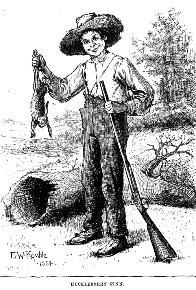
tidy_huck

# A tibble: 55,198 x 3
   document term         count
   <chr>    <chr>        <dbl>
 1 1        finn             1
 2 1        huckleberry     1
 3 3        ago              1
 4 3        fifty            1
 5 3        forty            1
 6 3        mississippi      1
 7 3        scene            1
 8 3        the              1
 9 3        time             1
10 3        valley           1
# … with 55,188 more rows

Huck Finn joined to AFINN

huck_finn_join <- tidy_huck %>% 
  inner_join(afinn, by = c("term" = "word"))

 huck_finn_join

# A tibble: 4,849 x 6
   document       term count     value
      <chr>      <chr> <dbl>     <int>
 1       11 adventures     1         2
 2       11     matter     1         1
 3       14       lied     1        -2
 4       17       true     1         2
 5       20        hid     1        -1
 6       20       rich     1         2
# ... with 4,843 more rows

Using summarize()

sample_df

# A tibble: 2 x 6
  document  term count  score
     <dbl> <chr> <dbl>  <dbl>
1       22 judge     1     -3
2       22  took     1      1

sample_df %>%
  group_by(document) %>%
  summarize(total_score = sum(score))

# A tibble: 1 x 2
  document total_score
     <dbl>       <dbl>
1       22          -2

Using filter()

filter(huck_finn_join, document == 20)

# A tibble: 2 x 6
  document  term count score
     <chr> <chr> <dbl>  <int>
1       20   hid     1     -1
2       20  rich     1      2

Plutchik & NRC

Plutchik Wheel

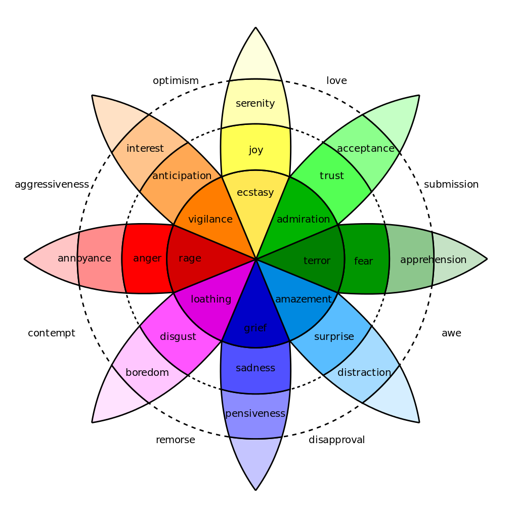
nrc <- get_sentiments("nrc")
head(nrc, 10)

# A tibble: 10 x 2
   word        sentiment
   <chr>       <chr>    
 1 abacus      trust    
 2 abandon     fear     
 3 abandon     negative 
 4 abandon     sadness  
 5 abandoned   anger    
 6 abandoned   fear     
 7 abandoned   negative 
 8 abandoned   sadness  
 9 abandonment anger    
10 abandonment fear

The Wonderful Wizard of NRC

Oz cover

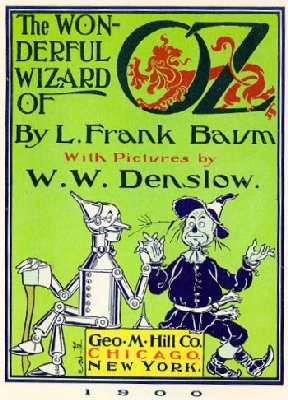
oz

# A tibble: 19,007 x 3
   document         term count
      <chr>        <chr> <dbl>
 1       1           the     1
 2       1        wizard     1
 3       1     wonderful     1
 4       6          baum     1
 5       6         frank     1
 6       10     contents     1
 7       12 introduction     1
 8       13      cyclone     1
 9       13          the     1
10       14      council     1
 # … with 18,997 more rows   1

%in% operator

x <- c("text", "mining", "python")

y <- c("text", "tm", "qdap", "R", "mining")

x %in% y

[1] TRUE TRUE FALSE

y %in% x

[1] TRUE FALSE FALSE FALSE TRUE

Let's practice!

Sentiment Analysis in R