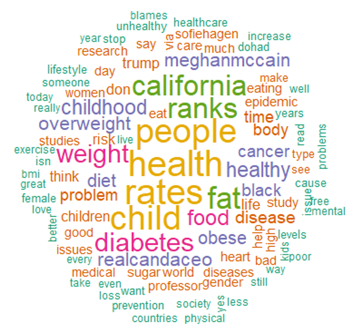
Visualize popular terms
Analyzing Social Media Data in R

Vivek Vijayaraghavan
Data Science Coach
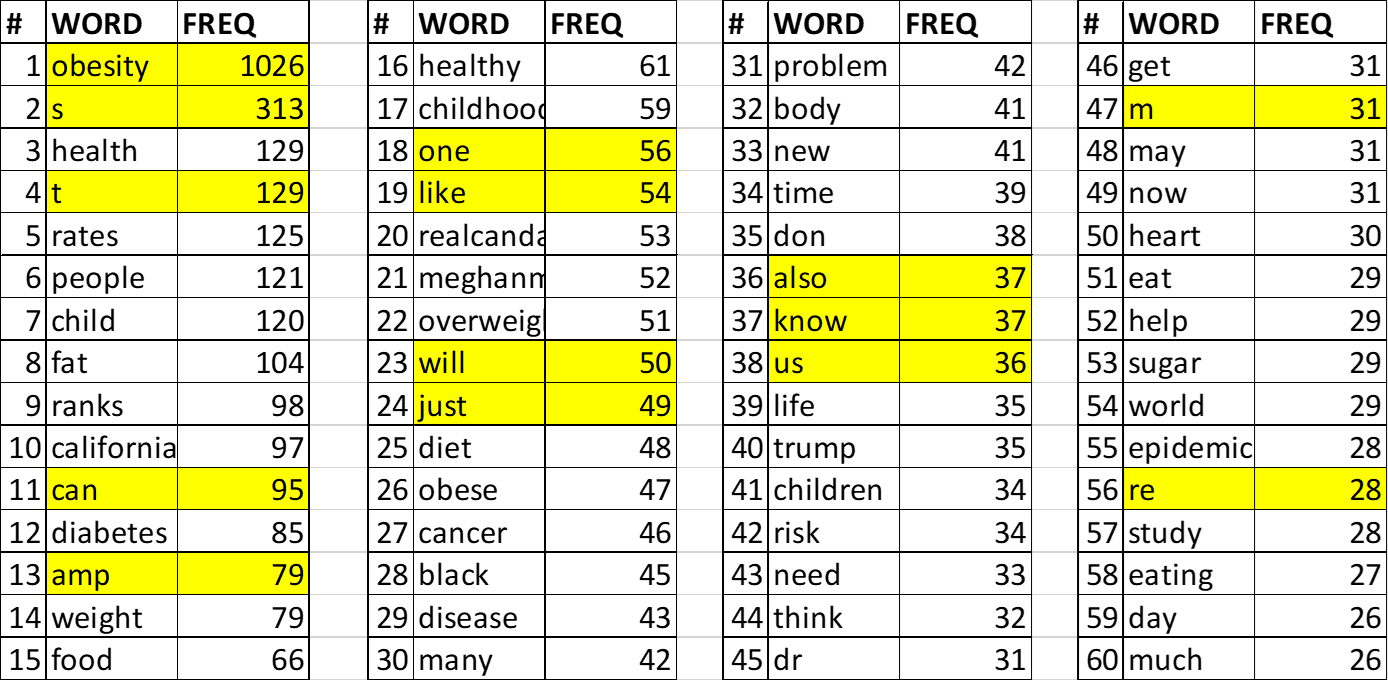
Term frequency
Term frequency after refining corpus
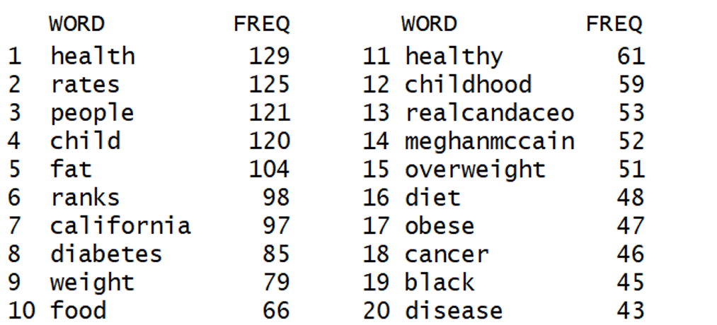
- Brand promoting an obesity management program can analyze these terms
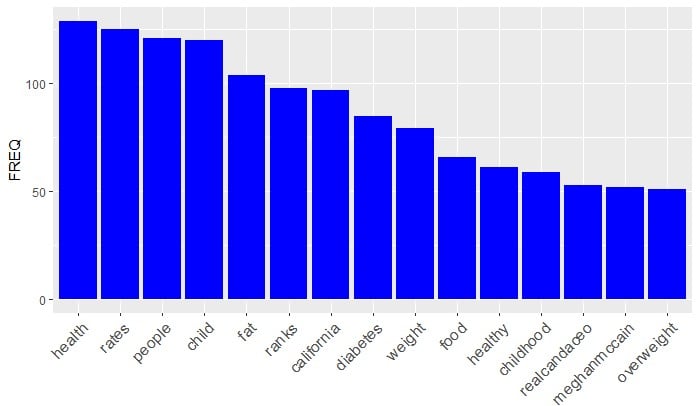
Bar plot of popular terms
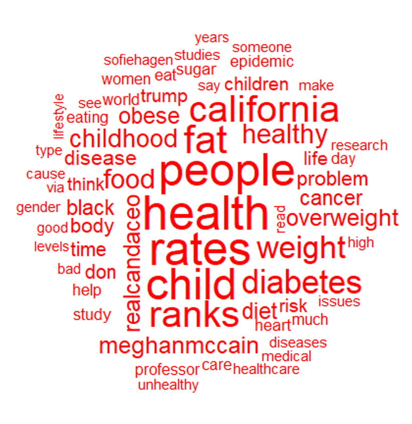
Word cloud based on min frequency
Colorful word cloud