Risk exposure and loss
Quantitative Risk Management in Python

Jamsheed Shorish
Computational Economist
A vacation analogy

Deciding between options


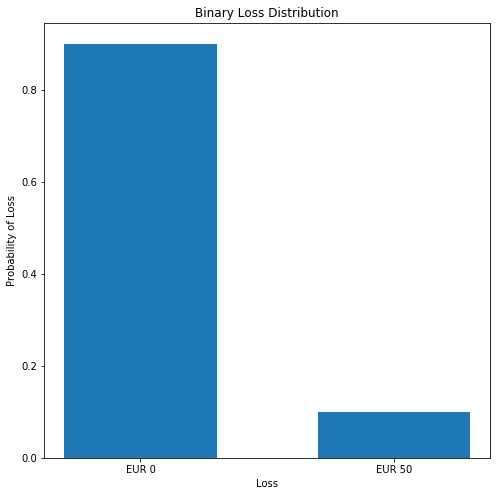
Loss distribution - discrete
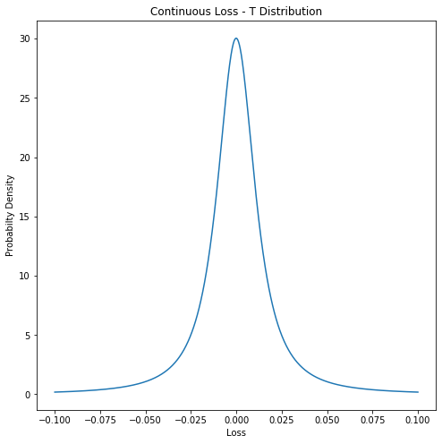
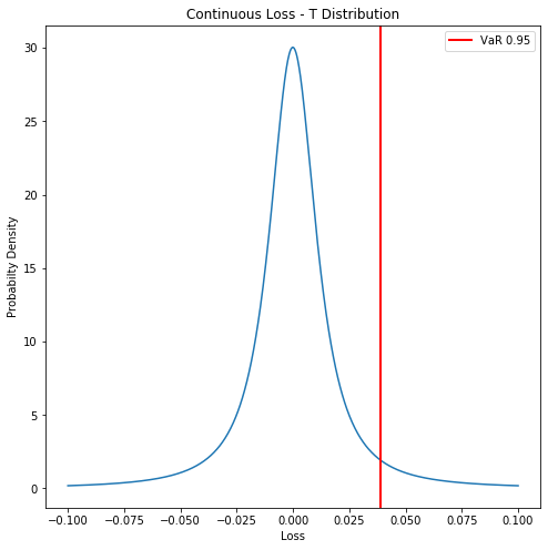
Loss distribution - continuous
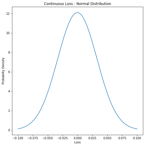
Loss distribution - continuous
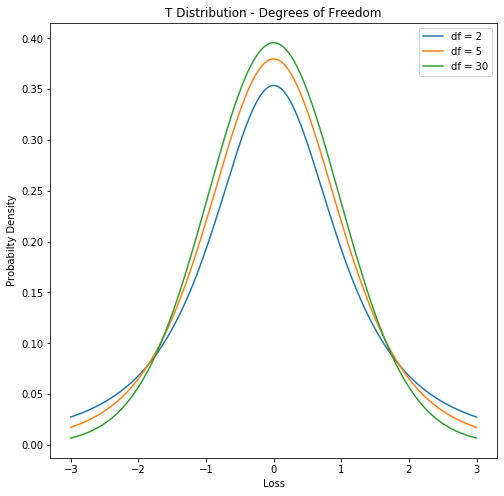
Primer: Student's t-distribution
T distribution in Python
T distribution in Python
Degrees of freedom