Theme flexibility

Introduction to Data Visualization with ggplot2

Rick Scavetta

Founder, Scavetta Academy

Ways to use themes

From scratch (last video)

Ways to use themes

From scratch (last video)
Theme layer object
Built-in themes
- ggplot2 or ggthemes packages
Built-in themes from other packages
Update/Set default theme

Defining theme objects

Useful when you have many plots
Provides consistency in style
Apply a specific theme everywhere

Defining theme objects

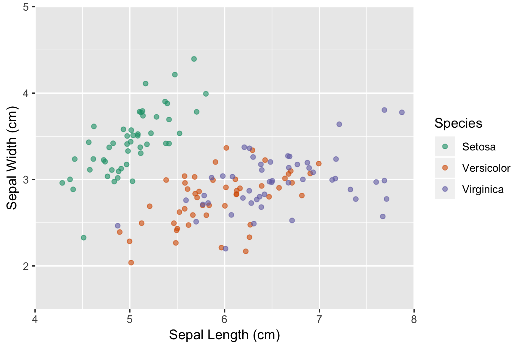
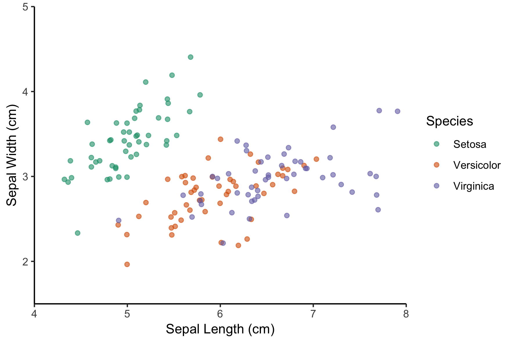
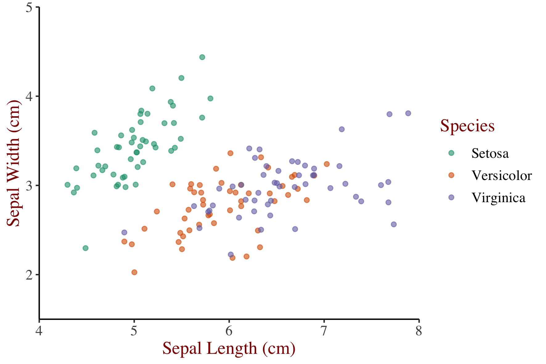
z <- ggplot(iris, aes(x = Sepal.Length, y = Sepal.Width, color = Species)) + 
  geom_jitter(alpha = 0.6) +
  scale_x_continuous("Sepal Length (cm)", limits = c(4,8), expand = c(0,0)) +
  scale_y_continuous("Sepal Width (cm)", limits = c(1.5,5), expand = c(0,0)) +
  scale_color_brewer("Species", palette = "Dark2", labels = c("Setosa", "Versicolor", "Virginica"))

Defining theme objects

z + theme(text = element_text(family = "serif", size = 14),
          rect = element_blank(),
          panel.grid = element_blank(),
          title = element_text(color = "#8b0000"),
          axis.line = element_line(color = "black"))

Defining theme objects

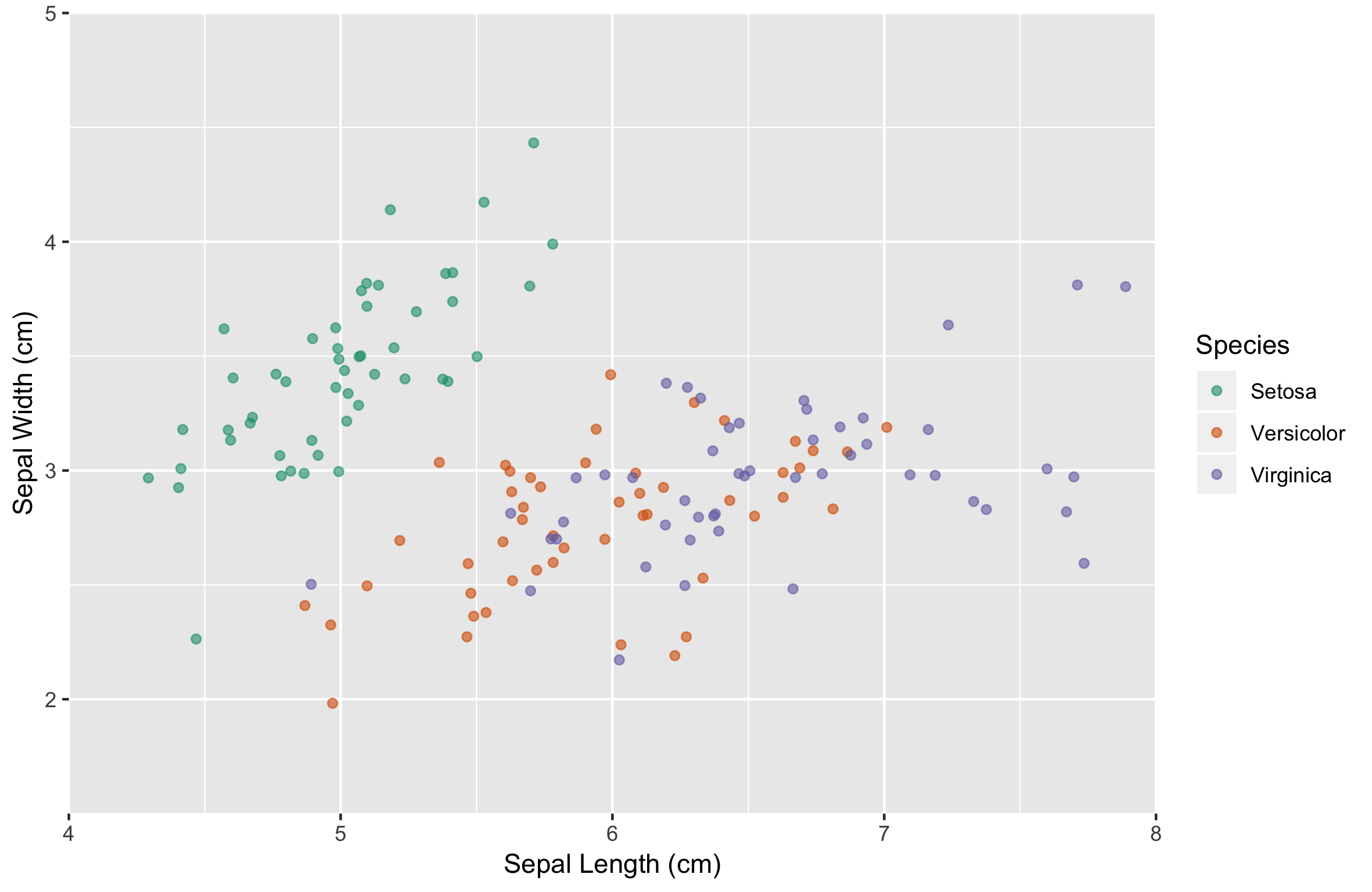
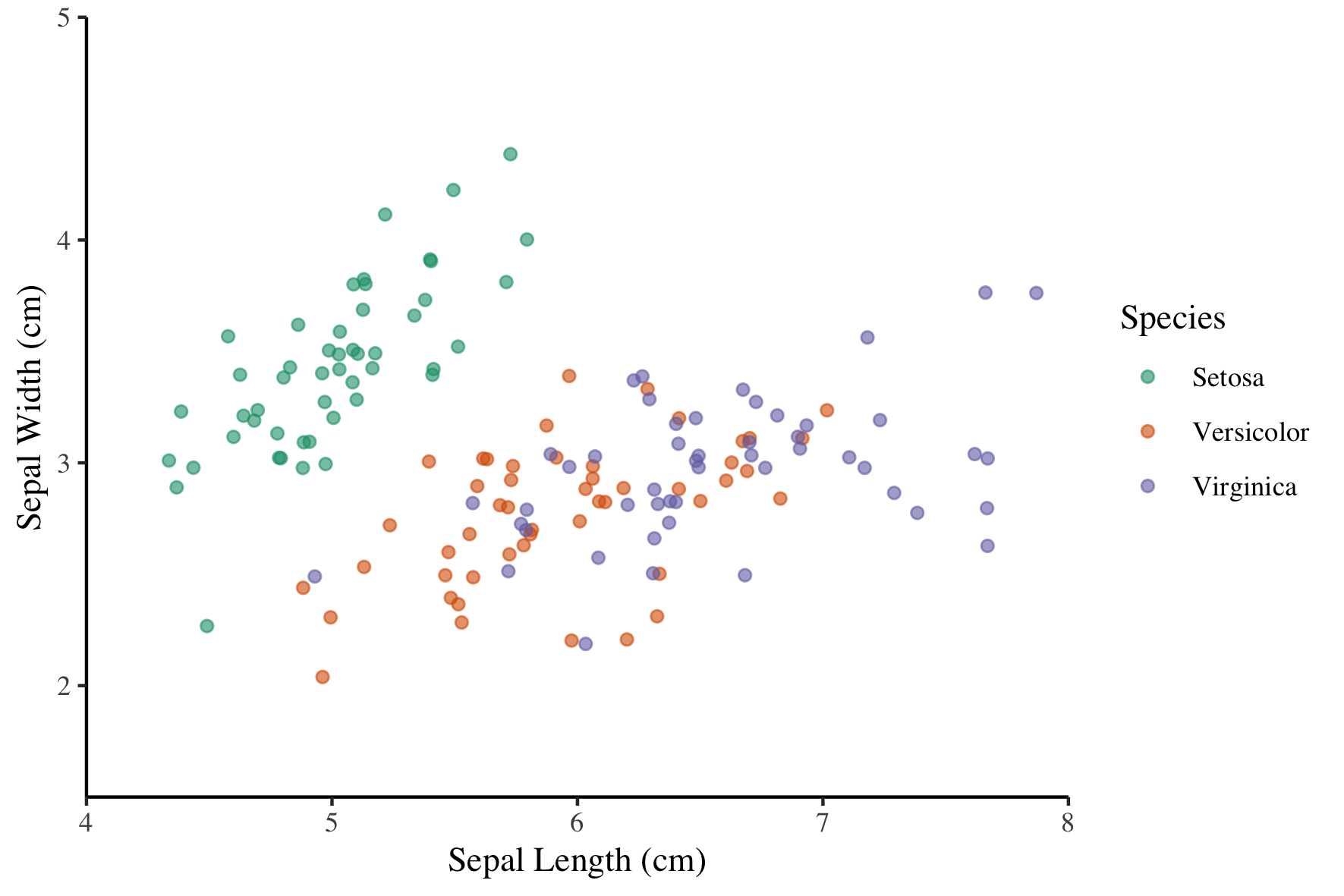
theme_iris <- theme(text = element_text(family = "serif", size = 14),
          rect = element_blank(),
          panel.grid = element_blank(),
          title = element_text(color = "#8b0000"),
          axis.line = element_line(color = "black"))

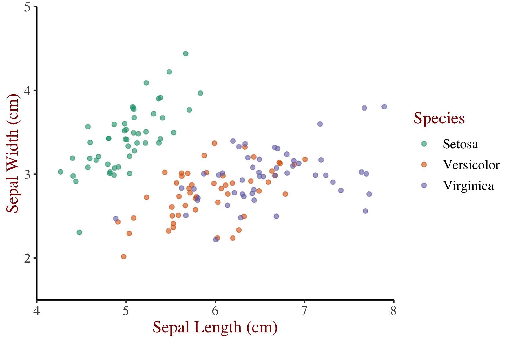
Reusing theme objects

z + theme_iris

Reusing theme objects

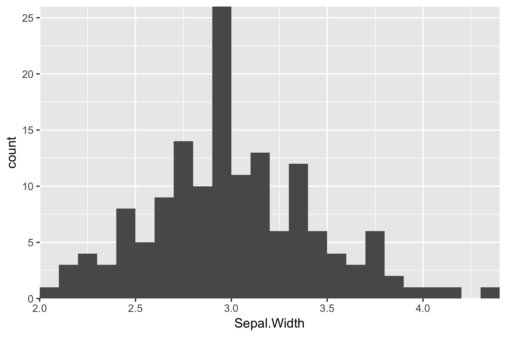
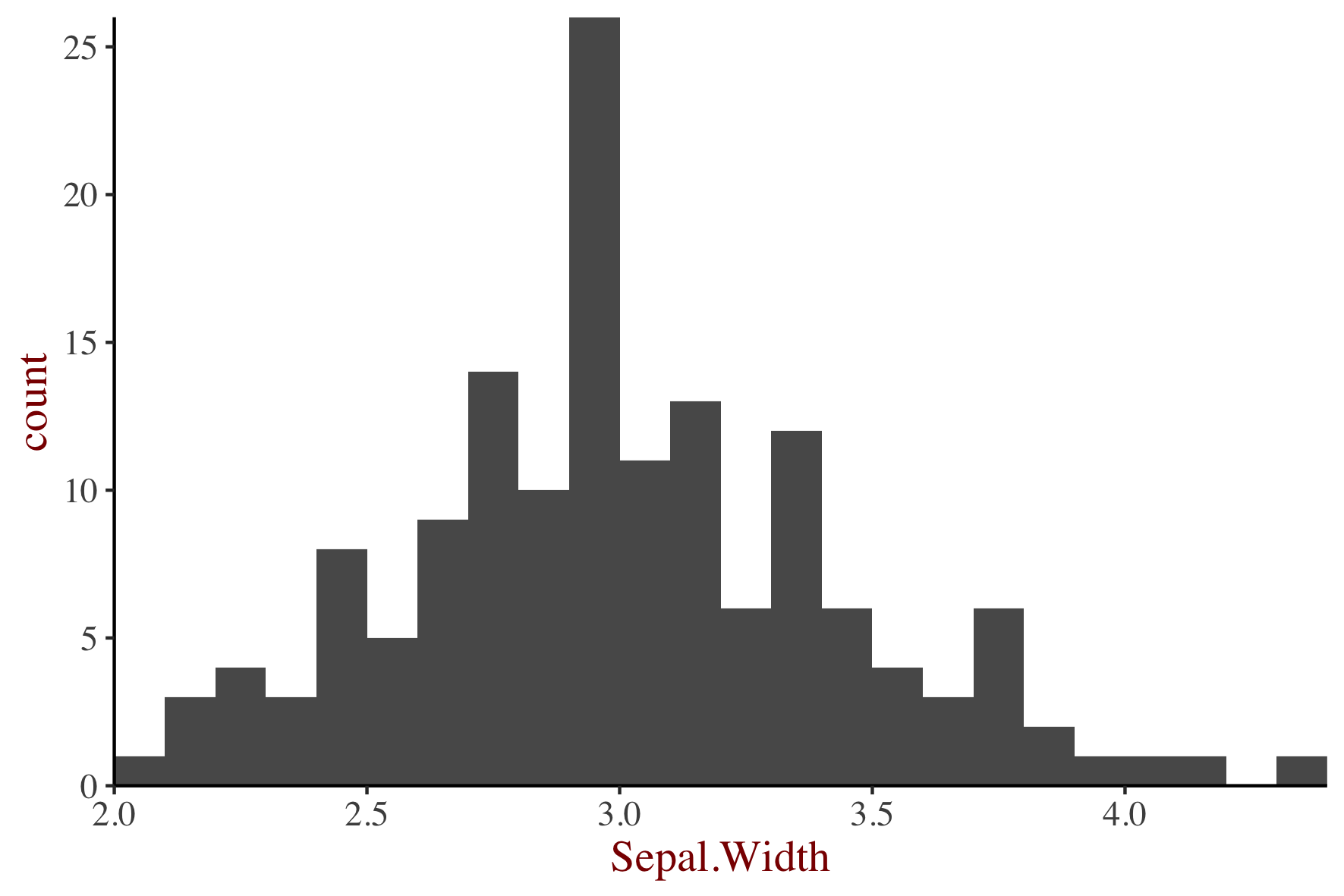
m <- ggplot(iris, aes(x = Sepal.Width)) + 
    geom_histogram(binwidth = 0.1,
                   center = 0.05)
m

Reusing theme objects

m +
  theme_iris

Reusing theme objects

m + 
  theme_iris +
  theme(axis.line.x = element_blank())

Ways to use themes

From scratch (last video)
Theme layer object
Built-in themes
- ggplot2 or ggthemes packages
Built-in themes from other packages
Update/Set default theme

Using built-in themes

Use theme_*() functions to access built-in themes.

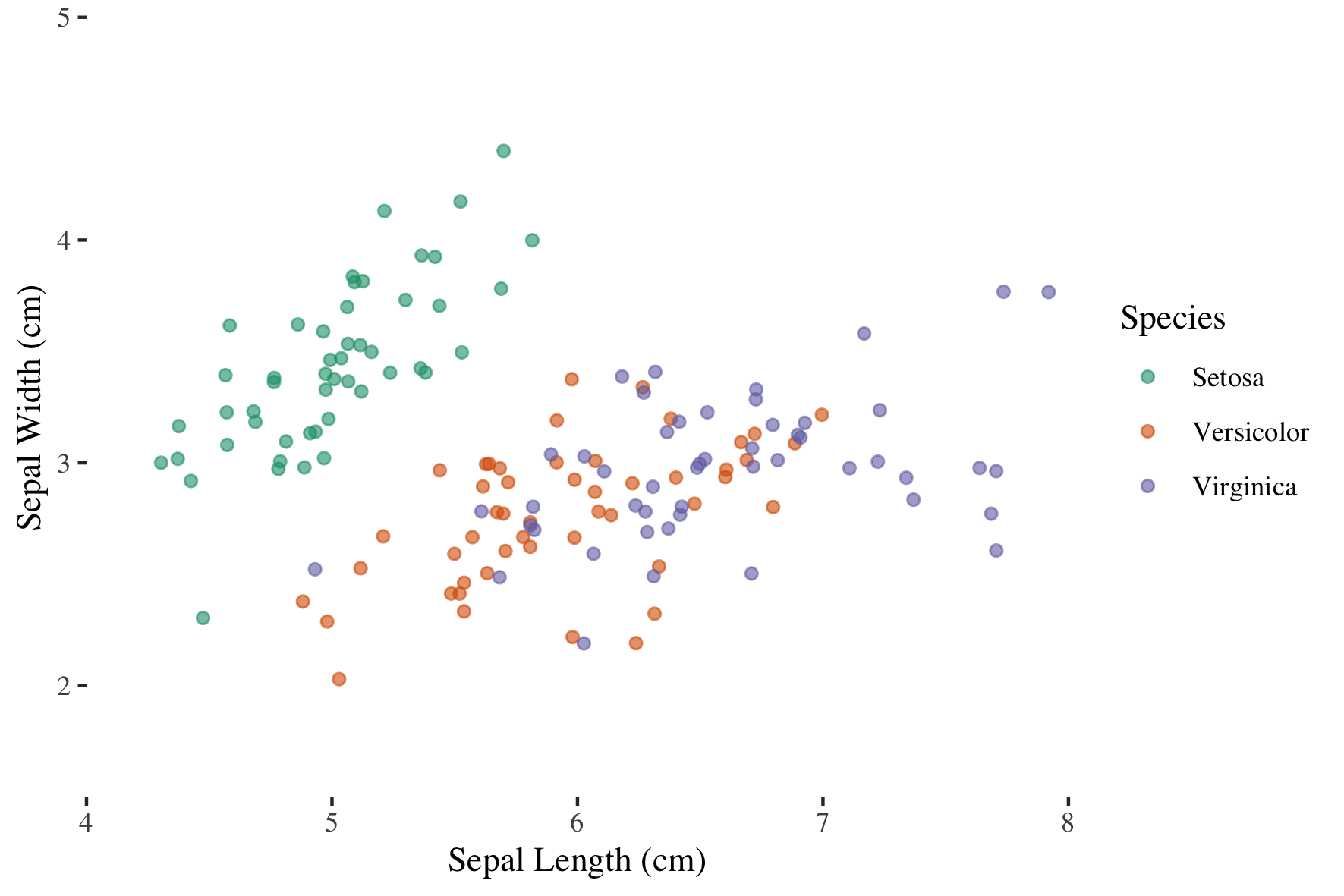
z + 
  theme_classic()

Using built-in themes

Use theme_*() functions to access built-in themes.

z + 
  theme_classic() +
  theme(text = element_text(family = "serif"))

Ways to use themes

From scratch (last video)
Theme layer object
Built-in themes
- ggplot2 or ggthemes packages
Built-in themes from other packages
Update/Set default theme

The ggthemes package

Use the ggthemes package for more functions.

library(ggthemes)
z + 
  theme_tufte()

Ways to use themes

From scratch (last video)
Theme layer object
Built-in themes
- ggplot2 or ggthemes packages
Built-in themes from other packages
Update/Set default theme

Updating themes

original <- theme_update(text = element_text(family = "serif", size = 14),
                         rect = element_blank(),
                         panel.grid = element_blank(),
                         title = element_text(color = "#8b0000"),
                         axis.line = element_line(color = "black"))

Updating themes

Setting themes

theme_set(original)

# Alternatively
# theme_set(theme_grey())

Let's practice!

Introduction to Data Visualization with ggplot2