The facets layer

Intermediate Data Visualization with ggplot2

Rick Scavetta

Founder, Scavetta Academy

Facets

Straight-forward yet useful
Concept of Small Multiples
- Popularized by Edward Tufte
- Visualization of Quantitative Information, 1983

iris.wide

p <- ggplot(iris.wide, aes(x = Length, 
                           y = Width, 
                           ccolorol = Part)) +
  geom_jitter(alpha = 0.7) +
  scale_color_brewer(palette = "Set1") +
  coord_fixed()

p

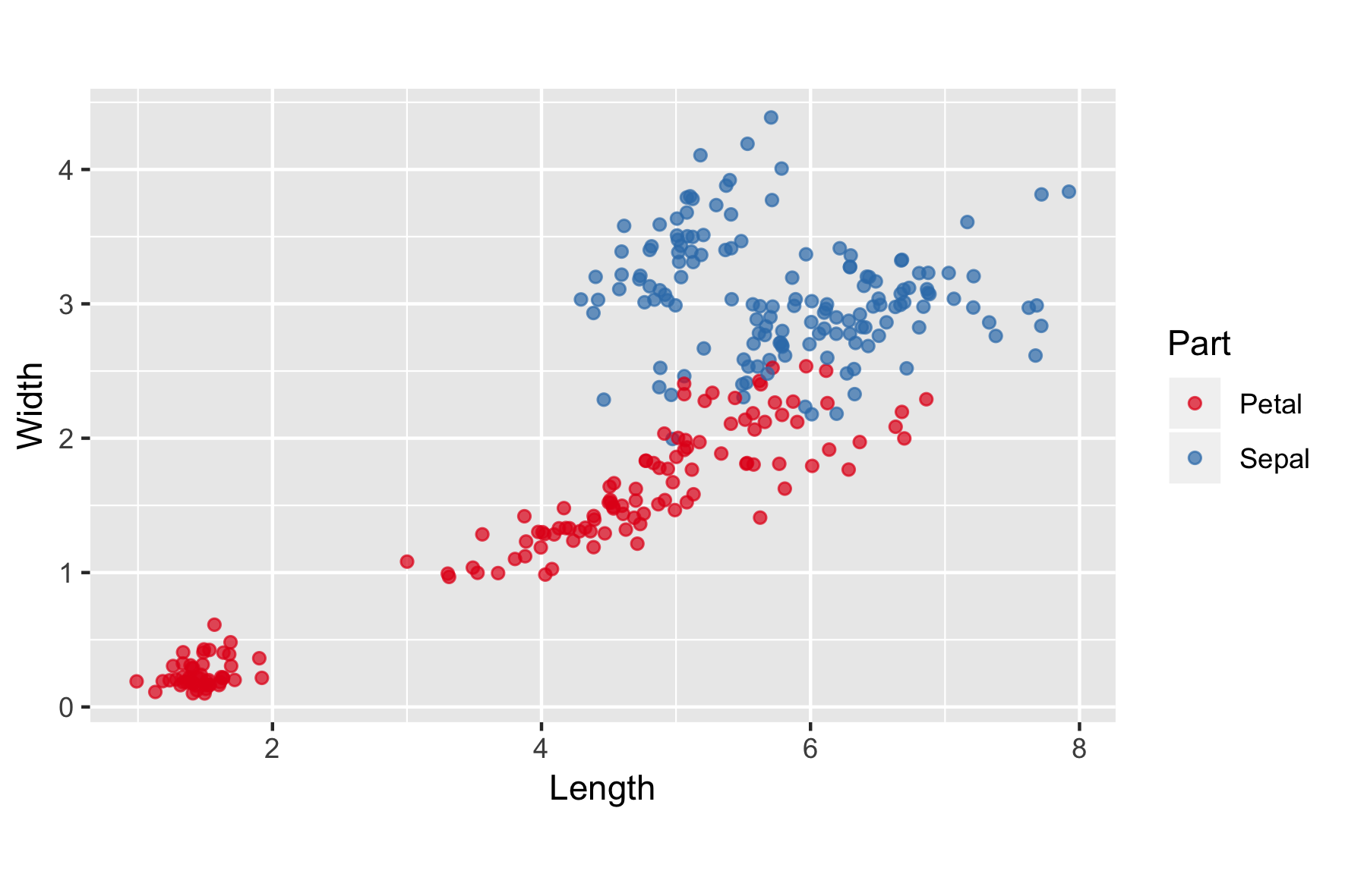
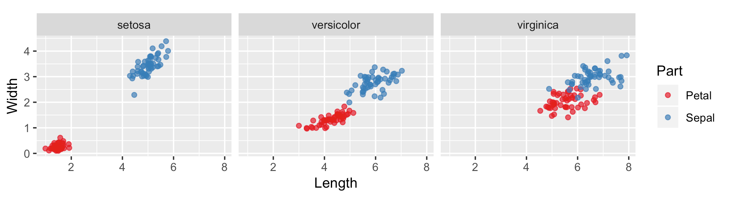
iris.wide & facet_grid()

p <- ggplot(iris.wide, aes(x = Length, y = Width, color = Part)) +
  geom_jitter(alpha = 0.7) +
  scale_color_brewer(palette = "Set1") +
  coord_fixed()
p + facet_grid(cols = vars(Species))

Formula notation

p <- ggplot(iris.wide, aes(x = Length, y = Width, color = Part)) +
  geom_jitter(alpha = 0.7) +
  scale_color_brewer(palette = "Set1") +
  coord_fixed()
p + facet_grid(. ~ Species)

iris.wide2

ggplot(iris.wide2, aes(x = Part, y = setosa, color = Measure)) +
  geom_jitter()
ggplot(iris.wide2, aes(x = Part, y = versicolor, color = Measure)) +
  geom_jitter()  
ggplot(iris.wide2, aes(x = Part, y = virginica, color = Measure)) +
  geom_jitter()

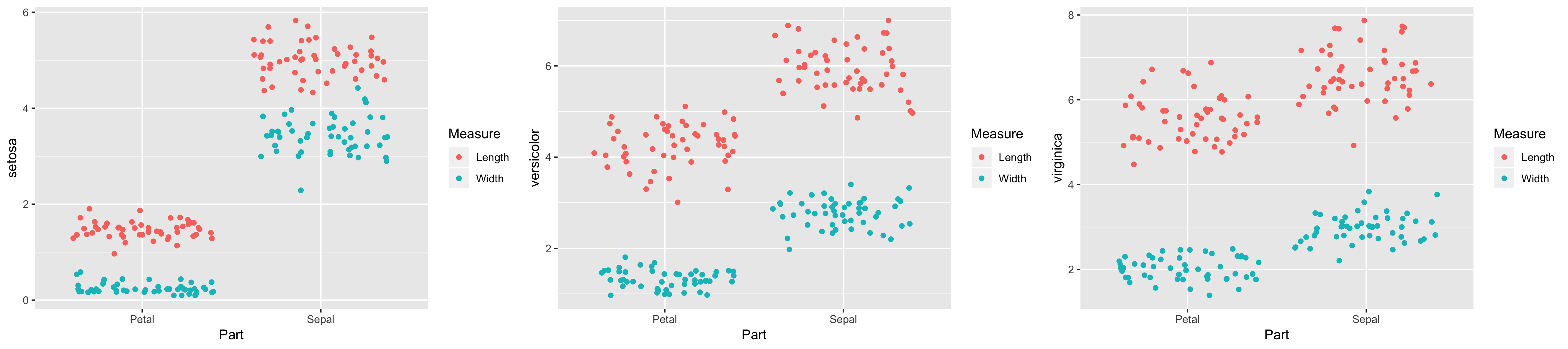
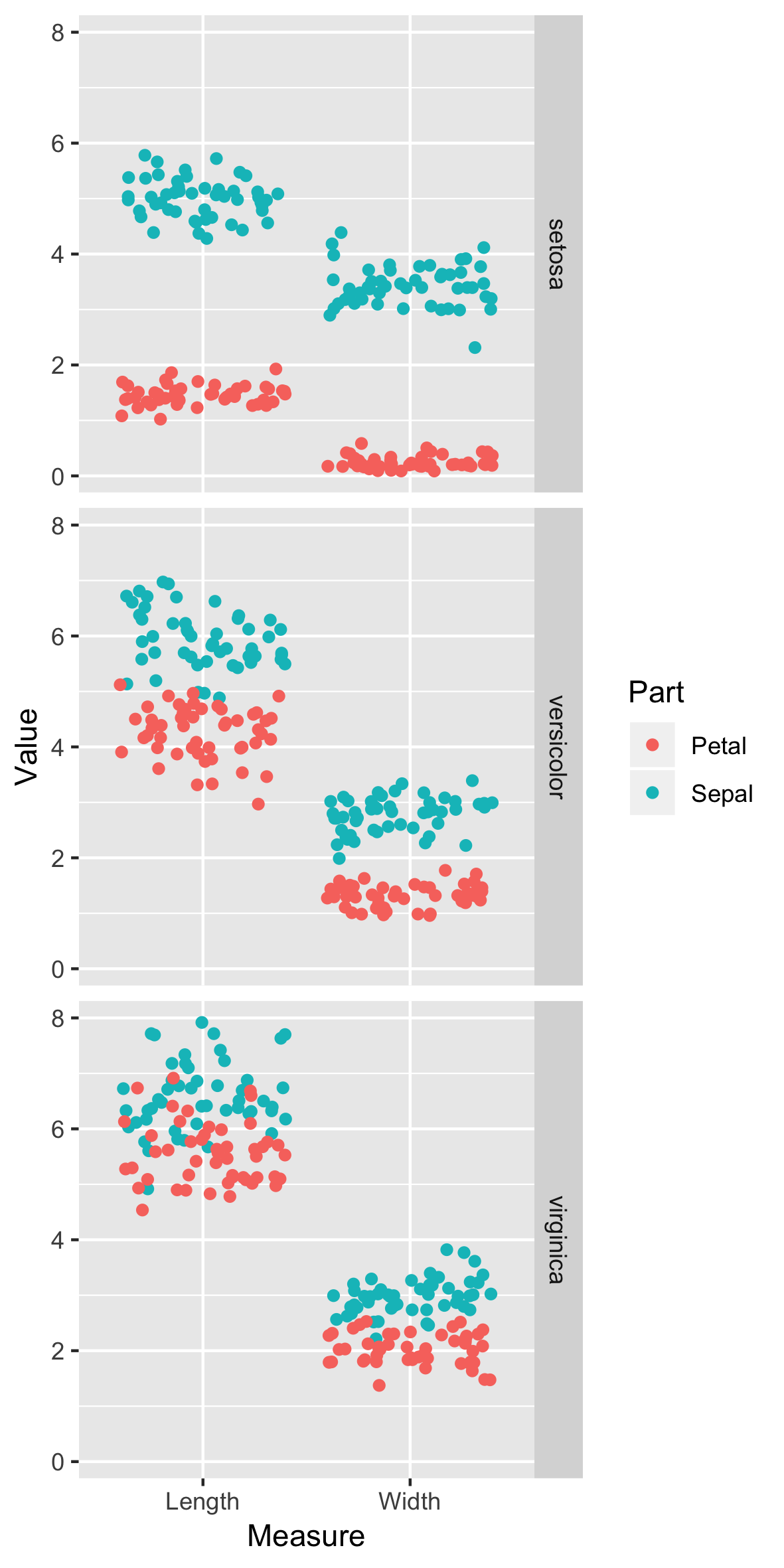
iris.tidy

ggplot(iris.tidy, aes(x = Measure, y = Value, color = Part)) +
  geom_jitter() +
  facet_grid(cols = vars(Species))

iris.tidy faceting done wrong:

ggplot(iris.tidy, aes(x = Measure, 
                      y = Value, 
                      color = Part)) +
  geom_jitter() +
  facet_grid(rows = vars(Species))

Other options

Split according to rows and columns

Let's practice!

Intermediate Data Visualization with ggplot2