Multiple imputation by bootstrapping
Handling Missing Data with Imputations in R

Michal Oleszak
Machine Learning Engineer
Uncertainty from imputation
- Imputation is typically a first step before analysis or modeling.
- Missing values are estimated with some uncertainty.
- This uncertainty should be accounted for in any analyses carried out on imputed data.
In almost half of the studies, key results disappear
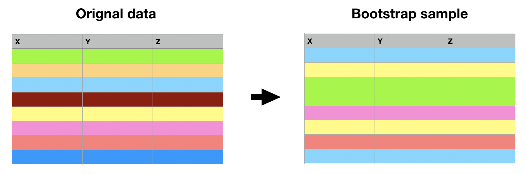
Bootstrap
Bootstrapping = sampling rows with replacement to get original-size data
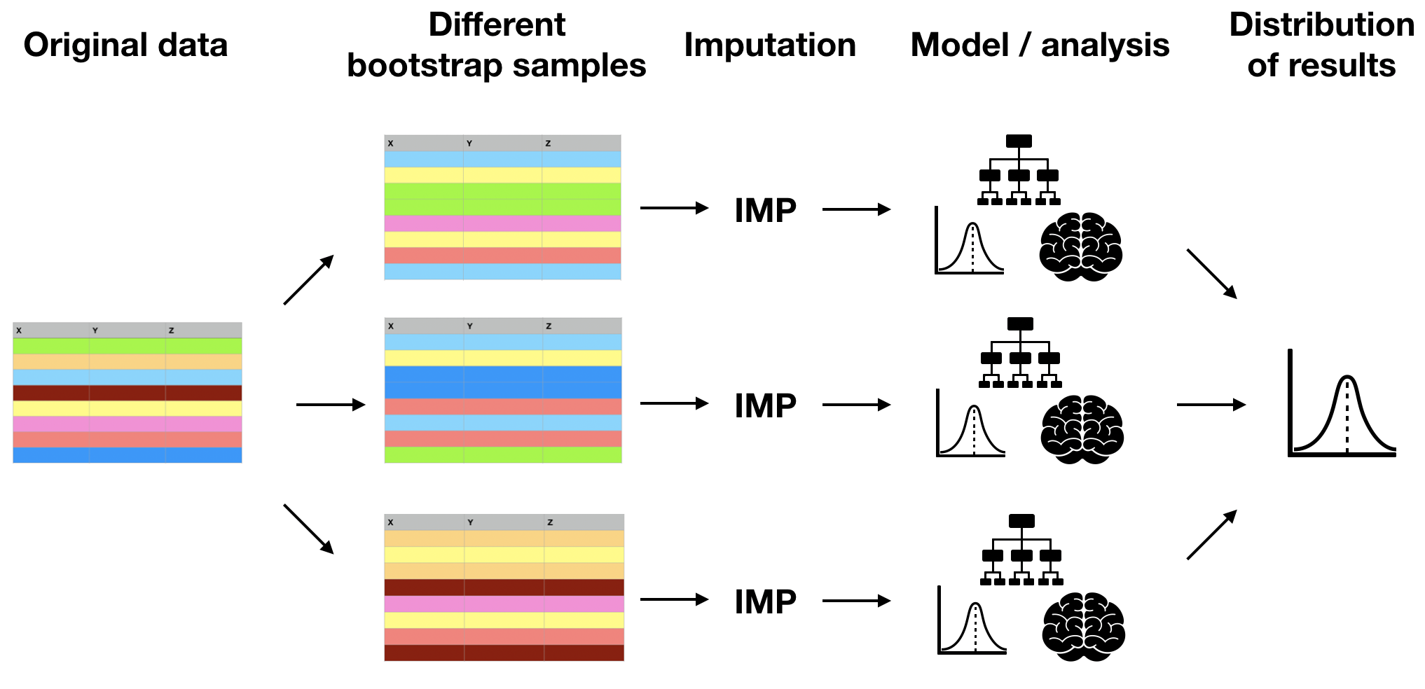
Multiple imputation by bootstrapping
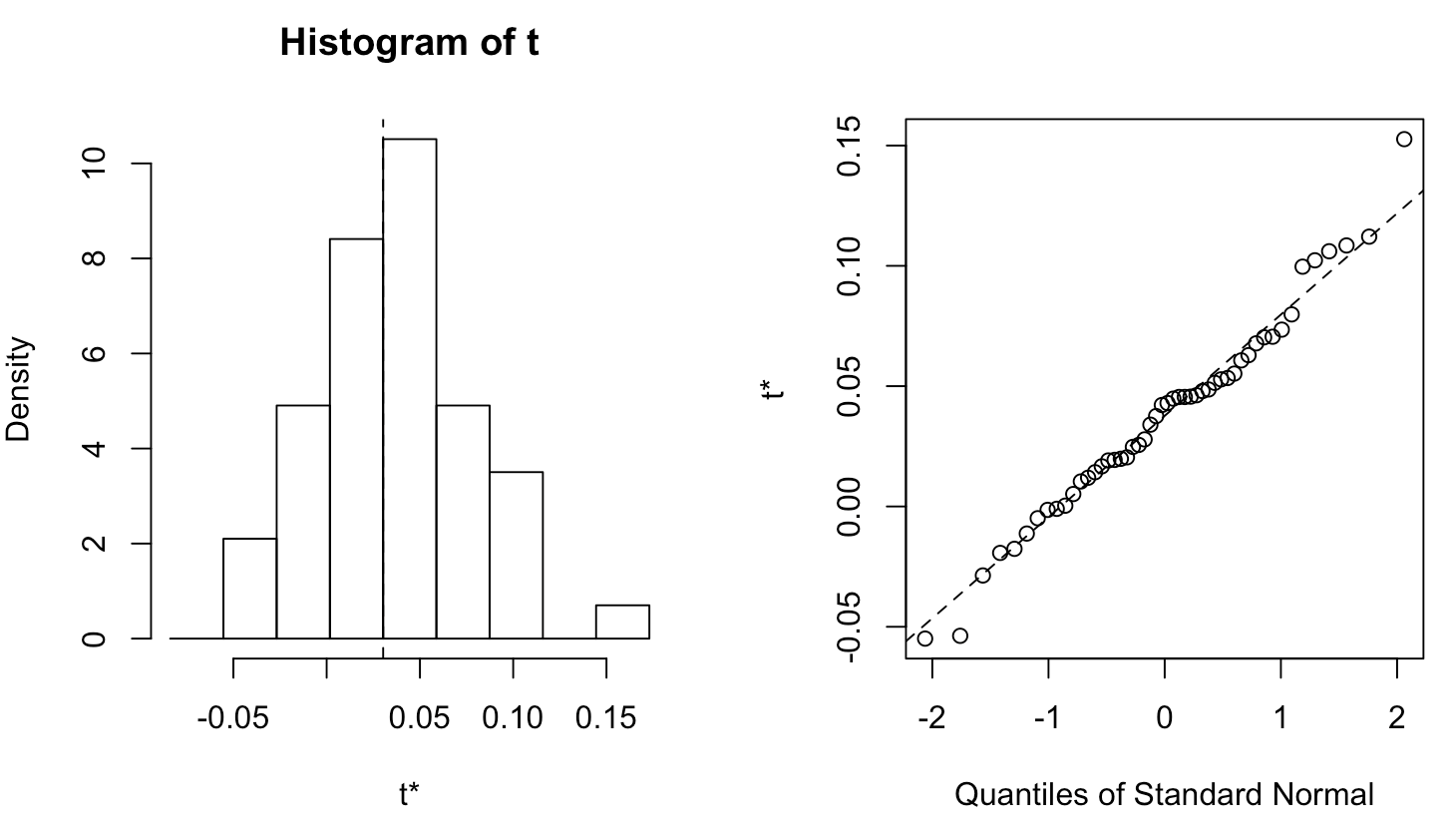
Plotting bootstrap results
plot(boot_results)