Random future lifetime

Life Insurance Products Valuation in R

Katrien Antonio, Ph.D.

Professor, KU Leuven and University of Amsterdam

The random future lifetime

$(x)$ denotes an individual aged $x$ at this moment, with $x \geq 0$.
The random variable $T_x$ is the future lifetime of $(x)$.
Thus, age at death of $(x)$ is $x + T_x$.

The life table in R

Human Mortality Database (HMD, www.mortality.org).
life_table contains the period life table for males in Belgium of 2013.

head(life_table, 10)

   age      qx     lx  dx    ex
1    0 0.00381 100000 381 77.95
2    1 0.00047  99619  47 77.24
3    2 0.00019  99572  19 76.28
4    3 0.00015  99553  15 75.30
5    4 0.00013  99538  13 74.31
6    5 0.00010  99525  10 73.32
7    6 0.00011  99514  11 72.32
8    7 0.00008  99504   8 71.33
9    8 0.00011  99496  11 70.34
10   9 0.00008  99485   8 69.34

Mortality rates and survival probabilities

The one-year probability of dying

$$ q_x = \text{Pr}(T_x \leq 1). $$

$\quad \;$ $q_x$ is the mortality rate at age $x$.
The one-year probability of surviving

$$ p_x = \text{Pr}(T_x > 1). $$
Thus, $p_x = 1 - q_x$.

Mortality rates of Belgian sportsmen in R

Eden Hazard is a Belgian footballer who plays for Chelsea and is 27 years old.

age <- life_table$age
qx <- life_table$qx
qx[age == 27]

0.00062

qx[27 + 1]

0.00062

Eddy Merckx is a Belgian cyclist who won the Tour de France 5 times and is 72.

qx[age == 72]

0.02631

qx[72 + 1]

0.02631

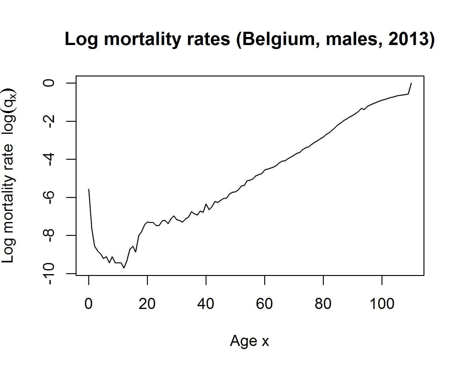
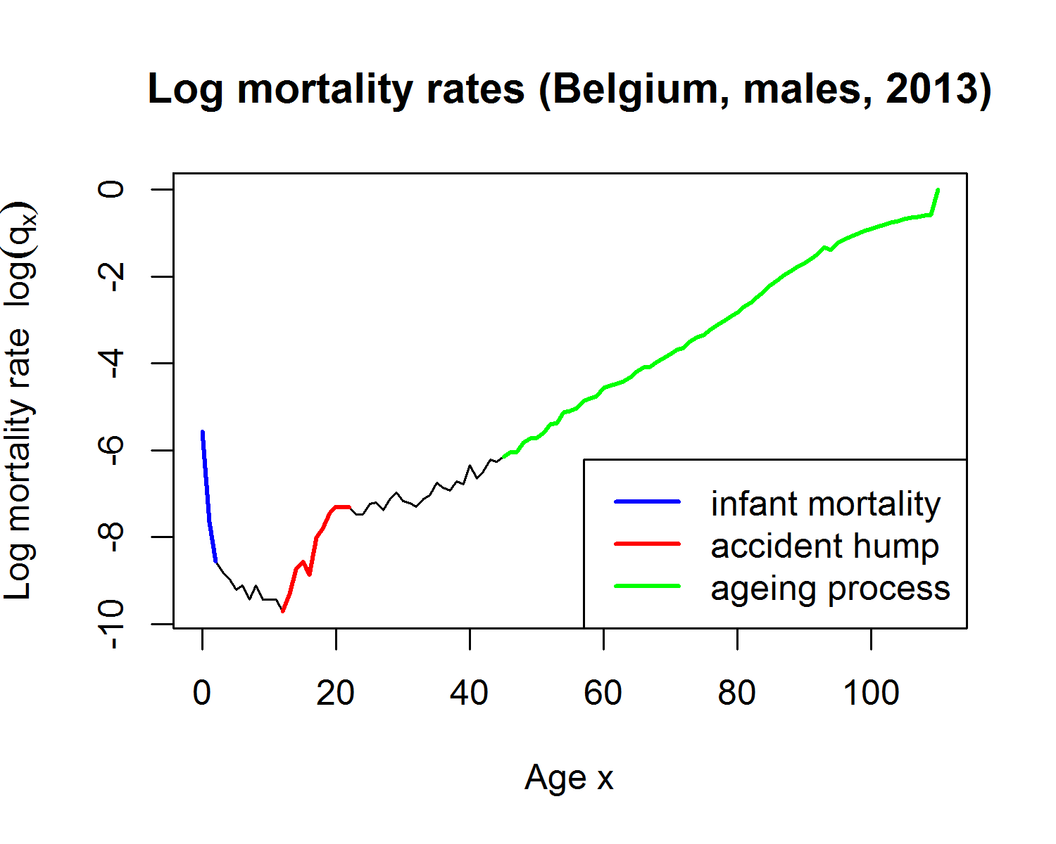
Picturing Belgian mortality rates $q_x$ in R

plot(age, log(qx), main = "Log mortality rates (Belgium, males, 2013)",
     xlab = "Age x", ylab = expression(paste("Log mortality rate ", log(q[x]))), 
     type = "l")

The life expectancy

The (complete) expected future lifetime of $(x)$ is $E[T_x]$
For Eden Hazard who is 27 years old:

ex <- life_table$ex
ex[27 + 1]

51.74

For Eddy Merckx who is 72 years old:

ex[72 + 1]

12.67

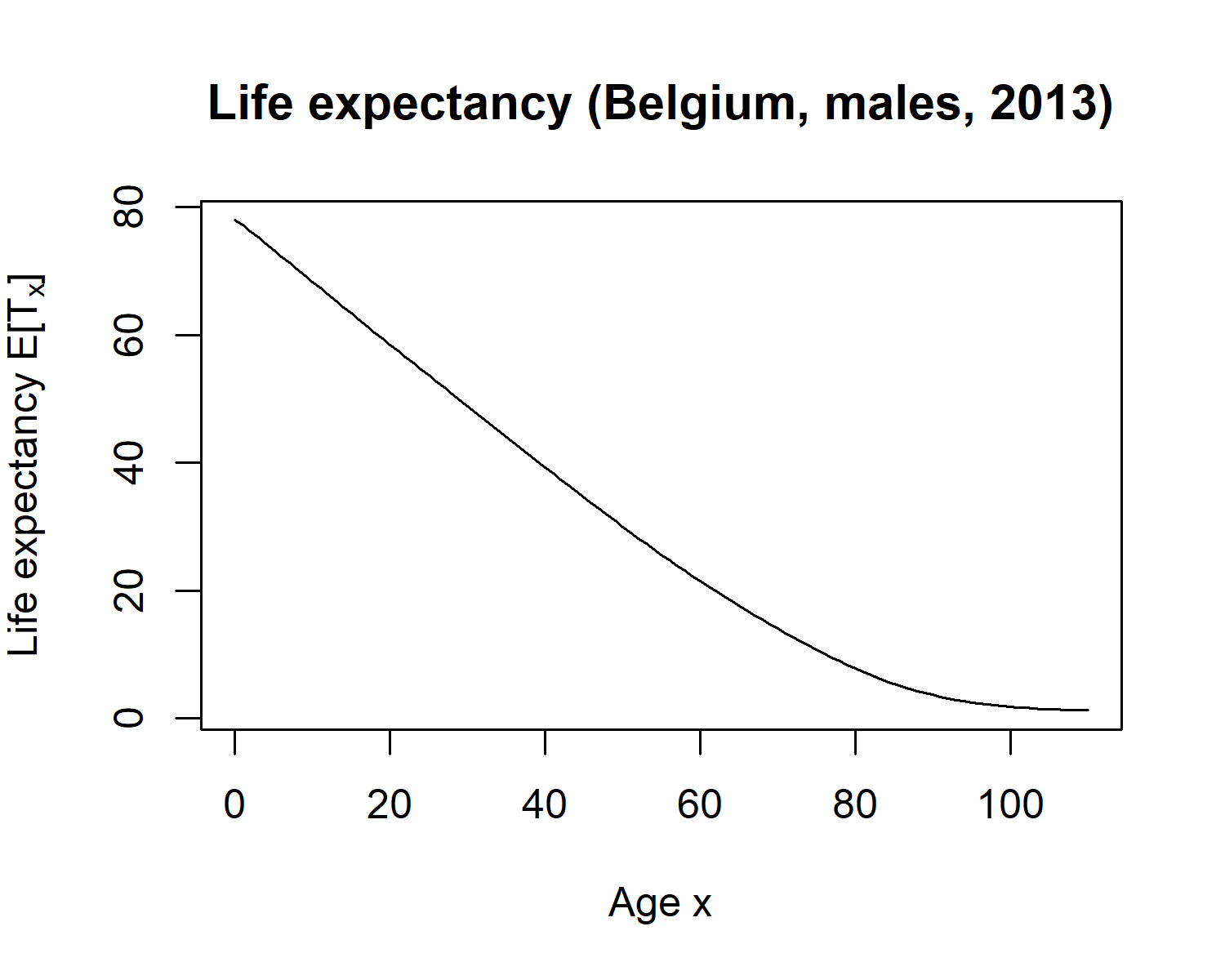
Picturing the life expectancy in R

plot(age, ex, main = "Life expectancy (Belgium, males, 2013)", xlab = "Age x", 
     ylab = expression(paste("Life expectancy E[", T[x], "]")), type = "l")

Let's practice!

Life Insurance Products Valuation in R