Comparing sampling and bootstrap distributions

Sampling in R

Richie Cotton

Data Evangelist at DataCamp

Coffee focused subset

set.seed(19790801)
coffee_sample <- coffee_ratings %>%
  select(variety, country_of_origin, flavor) %>%
  rowid_to_column() %>% 
  slice_sample(n = 500)
glimpse(coffee_sample)

Rows: 500
Columns: 4
$ rowid             <int> 10, 278, 458, 622, 131, 385, 1292, 47, 904, 1020, 5...
$ variety           <chr> "Other", "Bourbon", NA, "Caturra", "Caturra", "Yell...
$ country_of_origin <chr> "Ethiopia", "Guatemala", "Colombia", "Thailand", "C...
$ flavor            <dbl> 8.58, 7.75, 7.75, 7.50, 8.00, 7.83, 7.17, 8.08, 7.3...

The bootstrap of mean coffee flavors

mean_flavors_1000 <- replicate(
  n = 1000,
  expr = coffee_sample %>%
    slice_sample(prop = 1, replace = TRUE) %>%
    summarize(mean_flavor = mean(flavor, na.rm = TRUE)) %>%
    pull(mean_flavor)
)
bootstrap_distn <- tibble(
  resample_mean = mean_flavors_1000
)

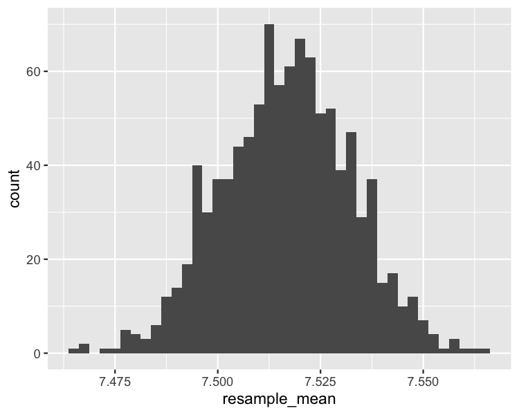
Mean flavor bootstrap distribution

 ggplot(bootstrap_distn, aes(resample_mean)) +
  geom_histogram(binwidth = 0.0025)

A histogram of the bootstrap distribution.

Sample, bootstrap distribution, population means

Sample mean

coffee_sample %>% 
  summarize(mean_flavor = mean(flavor)) %>% 
  pull(mean_flavor)

7.5163

Estimated population mean

bootstrap_distn %>% 
  summarize(mean_mean_flavor = mean(resample_mean)) %>% 
  pull(mean_mean_flavor)

7.5167

True population mean

coffee_ratings %>% 
  summarize(mean_flavor = mean(flavor)) %>% 
  pull(mean_flavor)

7.5260

Interpreting the means

The bootstrap distribution mean is usually almost identical to the sample mean.
It may not be a good estimate of the population mean.
Bootstrapping cannot correct biases due to differences between your sample and the population.

Sample sd vs bootstrap distribution sd

Sample standard deviation

coffee_focus %>% 
  summarize(sd_flavor = sd(flavor)) %>% 
  pull(sd_flavor)

0.3525

Estimated population standard deviation?

bootstrap_distn %>% 
  summarize(sd_mean_flavor = sd(resample_mean)) %>% 
  pull(sd_mean_flavor)

0.01572

Sample, bootstrap dist'n, pop'n standard deviations

Sample standard deviation

coffee_focus %>% 
  summarize(sd_flavor = sd(flavor)) %>% 
  pull(sd_flavor)

0.3525

Estimated population standard deviation

standard_error <- bootstrap_distn %>%
  summarize(sd_mean_flavor = sd(resample_mean)) %>% 
  pull(sd_mean_flavor)

standard_error * sqrt(500)

0.3515

True standard deviation

coffee_ratings %>%
  summarize(sd_flavor = sd(flavor)) %>%
  pull(sd_flavor)

0.3414

Standard error is the standard deviation of the statistic of interest.

Standard error times square root of sample size estimates the population standard deviation.

Interpreting the standard errors

Estimated standard error is the standard deviation of the bootstrap distribution for a sample statistic.
The bootstrap distribution standard error times the square root of the sample size estimates the standard deviation in the population.

Let's practice!

Sampling in R