Standard errors and the Central Limit Theorem

Sampling in R

Richie Cotton

Data Evangelist at DataCamp

Sampling distribution of mean cup points

A histogram of approximate sampling distribution of mean cup points with a sample size of five.

A histogram of approximate sampling distribution of mean cup points with a sample size of 20.

A histogram of approximate sampling distribution of mean cup points with a sample size of 80.

A histogram of approximate sampling distribution of mean cup points with a sample size of 320.

Sampling in R

Consequences of the central limit theorem

  • Averages of independent samples have approximately normal distributions.

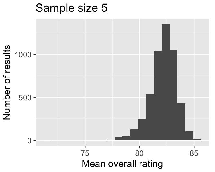
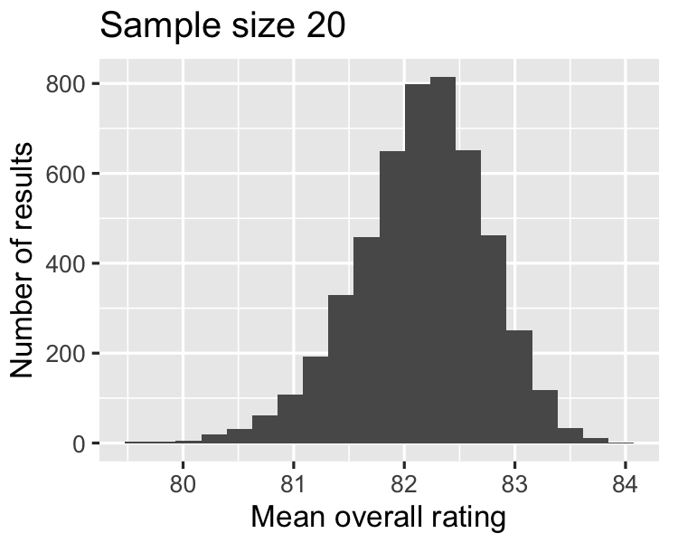
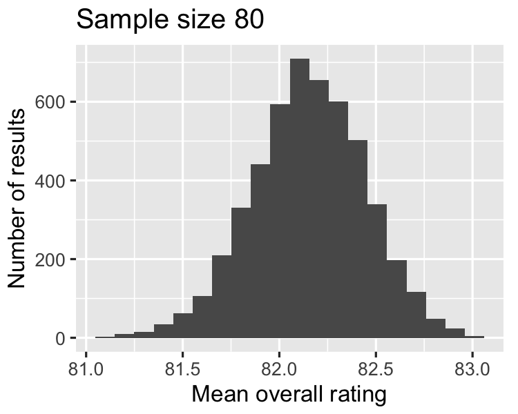
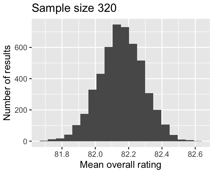
As the sample size increases,

  • the distribution of the averages gets closer to being normally distributed, and

  • the width of the sampling distribution gets narrower.

Sampling in R

Population & sampling distribution means

coffee_ratings %>%
  summarize(
    mean_cup_points = mean(total_cup_points)
  ) %>% 
  pull(mean_cup_points)
82.1512
Sample size Mean sample mean
5 82.1496
20 82.1610
80 82.1496
320 82.1521
Sampling in R

Population & sampling distribution standard deviations

coffee_ratings %>%
  summarize(
    sd_cup_points = sd(total_cup_points)
  ) %>%
  pull(sd_cup_points)
2.68686
Sample size Std dev sample mean
5 1.1929
20 0.6028
80 0.2865
320 0.1304
Sampling in R

Population mean over square root sample size

Sample size Std dev sample mean Calculation Result
5 1.1929 2.68686 / sqrt(5) 1.2016
20 0.6028 2.68686 / sqrt(20) 0.6008
80 0.2865 2.68686 / sqrt(80) 0.3004
320 0.1304 2.68686 / sqrt(320) 0.1502
Sampling in R

Let's practice!

Sampling in R

Preparing Video For Download...