Creating a sampling distribution

Sampling in R

Richie Cotton

Data Evangelist at DataCamp

Same code, different answer

coffee_ratings %>% 
  slice_sample(n = 30) %>% 
  summarize(mean_cup_points = mean(total_cup_points)) %>% 
  pull(mean_cup_points)

83.33

coffee_ratings %>% 
  slice_sample(n = 30) %>% 
  summarize(mean_cup_points = mean(total_cup_points)) %>% 
  pull(mean_cup_points)

82.59

coffee_ratings %>% 
  slice_sample(n = 30) %>% 
  summarize(mean_cup_points = mean(total_cup_points)) %>% 
  pull(mean_cup_points)

82.16

coffee_ratings %>% 
  slice_sample(n = 30) %>% 
  summarize(mean_cup_points = mean(total_cup_points)) %>% 
  pull(mean_cup_points)

82.25

Same code, 1000 times

mean_cup_points_1000 <- replicate(
  n = 1000,
  expr = coffee_ratings %>% 
    slice_sample(n = 30) %>% 
    summarize(
      mean_cup_points = mean(total_cup_points)
    ) %>% 
    pull(mean_cup_points)
)

   [1] 81.65 81.57 82.66 82.27 81.76 81.74 82.71
   [8] 82.20 80.43 82.45 82.29 82.63 82.28 82.11
  [15] 82.14 81.72 81.97 82.58 81.78 82.47 81.73
  [22] 82.78 82.14 82.39 81.69 82.36 82.64 82.68
  [29] 82.56 82.14 82.72 82.43 81.68 82.74 82.80
  [36] 82.12 82.31 81.02 82.83 81.71 82.25 82.11
  [43] 82.76 82.26 81.57 82.00 81.75 81.47 81.99
  [50] 82.68 82.05 82.43 82.40 82.66 80.78 82.43
  ...
 [967] 81.84 83.12 81.54 81.83 82.24 82.36 82.49
 [974] 82.05 82.08 81.98 82.45 82.04 81.42 83.06
 [981] 81.97 82.65 81.12 82.48 81.64 81.92 81.96
 [988] 81.71 81.96 81.78 82.30 81.76 82.46 82.43
 [995] 81.95 82.60 81.84 82.78 82.23 82.56

Preparing for plotting

library(tibble)
sample_means <- tibble(
  sample_mean = mean_cup_points_1000
)

# A tibble: 1,000 x 1
   sample_mean
         <dbl>
 1        83.3
 2        82.6
 3        82.2
 4        82.2
 5        81.7
 6        81.6
 7        82.7
 8        82.3
 9        81.8
10        81.7
# ... with 990 more rows

Distribution of sample means for size 30

ggplot(sample_means, aes(sample_mean)) +
  geom_histogram(binwidth = 0.1)

A sampling distribution is a distribution of several replicates of point estimates.

A histogram of sample means.

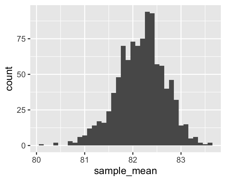
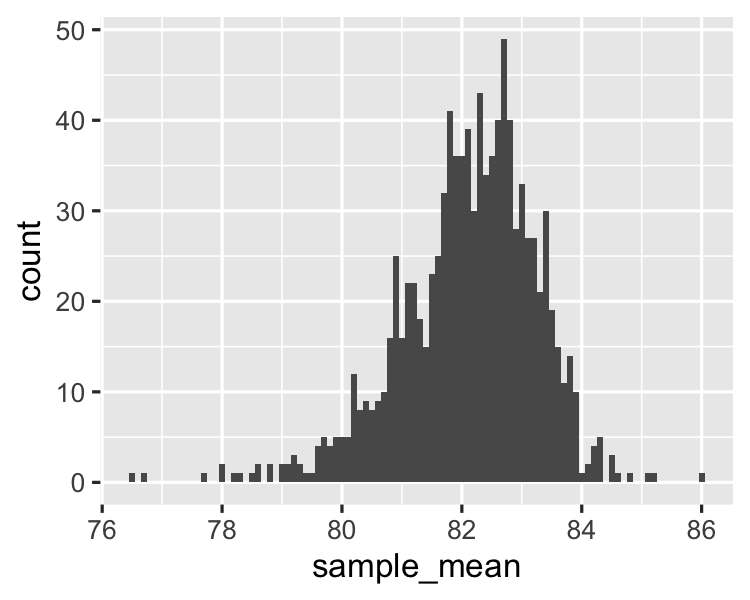
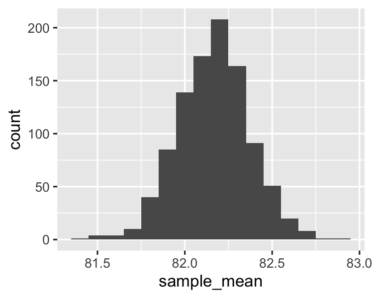
Different sample sizes

Sample size 6

A histogram of sample means with a sample size of six.

Sample size 150

A histogram of sample means with a sample size of 150.

Let's practice!

Sampling in R