Nesting data for modeling
Reshaping Data with tidyr

Jeroen Boeye
Head of Machine Learning, Faktion
USA Olympic performance
usa_olympic_df
# A tibble: 50 x 5
   country  year season n_participants n_medals
   <chr>   <dbl> <chr>           <int>    <int>
 1 USA      1896 Summer             14       20
 2 USA      1900 Summer             75       63
 3 USA      1904 Summer            524      394
 4 USA      1906 Summer             38       24
 5 USA      1908 Summer            122       65
 6 USA      1912 Summer            174      107
# ... with 44 more rows
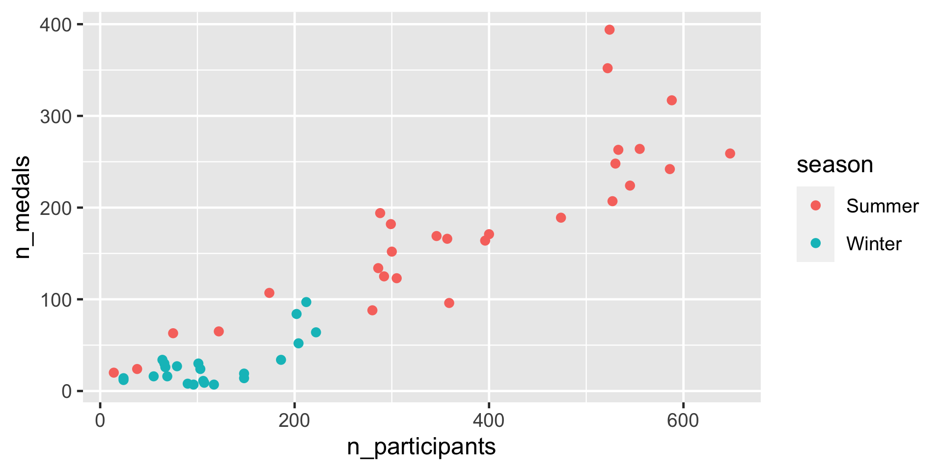
USA Olympic performance
usa_olympic_df %>%
  ggplot(aes(x = n_participants, y = n_medals, color = season))+
  geom_point()
Modeling the pattern
model <- lm(n_medals ~ n_participants + 0, data = usa_olympics_df)

model
Call:
lm(formula = n_medals ~ n_participants + 0, data = usa_olympics_df)

Coefficients:
n_participants
         0.463
Untidy model statistics
summary(model)
Call:
lm(formula = n_medals ~ n_participants + 0, data = usa_olympics_df)
Residuals:
    Min      1Q  Median      3Q     Max
-70.222 -36.175  -9.554   6.871 151.380
Coefficients:
               Estimate Std. Error t value Pr(>|t|)
n_participants  0.46302    0.01791   25.86   <2e-16 ***
--
Signif. codes:  0 '***' 0.001 '**' 0.01 '*' 0.05 '.' 0.1 ' ' 1
Residual standard error: 40.17 on 49 degrees of freedom
Multiple R-squared:  0.9317,    Adjusted R-squared:  0.9303
F-statistic: 668.5 on 1 and 49 DF,  p-value: < 2.2e-16
The broom package
broom::glance(model)
# A tibble: 1 x 11
  r.squared adj.r.squared sigma statistic  p.value    df logLik   AIC   BIC deviance df.residual
      <dbl>         <dbl> <dbl>     <dbl>    <dbl> <int>  <dbl> <dbl> <dbl>    <dbl>       <int>
1     0.932         0.930  40.2      668. 3.25e-30     1  -255.  514.  518.   79079.          49
broom::tidy(model)
# A tibble: 1 x 5
  term           estimate std.error statistic  p.value
  <chr>             <dbl>     <dbl>     <dbl>    <dbl>
1 n_participants    0.463    0.0179      25.9 3.25e-30
broom + dplyr + tidyr
usa_olympics_df %>%
  group_by(country) %>%
  nest()
# A tibble: 1 x 2
# Groups:   country [1]
  country data
  <chr>   <list>
1 USA     <tibble [50 × 4]>
Nested tibble & purrr::map()
usa_olympics_df %>%
  group_by(country) %>%
  nest() %>%
  mutate(fit = purrr::map(data, function(df) lm(n_medals ~ n_participants + 0, data = df)))
 # A tibble: 1 x 3
# Groups:   country [1]
  country data              fit
  <chr>   <list>            <list>
1 USA     <tibble [50 × 4]> <lm>
Working with nested tibbles
usa_olympics_df %>%
  group_by(country) %>%
  nest() %>%
  mutate(fit = purrr::map(data, function(df) lm(n_medals ~ n_participants + 0, data = df)),
         glanced = purrr::map(fit, broom::glance))
 # A tibble: 1 x 4
# Groups:   country [1]
  country data              fit    glanced
  <chr>   <list>            <list> <list>
1 USA     <tibble [50 × 4]> <lm>   <tibble [1 × 11]>
Unnesting model results
usa_olympics_df %>%
  group_by(country) %>%
  nest() %>%
  mutate(fit = purrr::map(data, function(df) lm(n_medals ~ n_participants + 0, data = df)),
         glanced = purrr::map(fit, broom::glance)) %>%
  unnest(glanced)
# A tibble: 1 x 14
# Groups:   country [1]
  country data              fit    r.squared adj.r.squared sigma statistic  p.value    df
  <chr>   <list>            <list>     <dbl>         <dbl> <dbl>     <dbl>    <dbl> <int>
1 USA     <tibble [50 × 4]> <lm>       0.932         0.930  40.2      668. 3.25e-30     1
# with 5 more variables: logLik <dbl>, AIC <dbl>, BIC <dbl> deviance <dbl>, df.residual <int>
Unnesting model results
usa_olympics_df %>%
  group_by(country) %>%
  nest() %>%
  mutate(fit = purrr::map(data, function(df) lm(n_medals ~ n_participants + 0, data = df)),
         tidied = purrr::map(fit, broom::tidy)) %>%
  unnest(tidied)
# A tibble: 1 x 8
# Groups:   country [1]
  country data              fit    term           estimate std.error statistic  p.value
  <chr>   <list>            <list> <chr>             <dbl>     <dbl>     <dbl>    <dbl>
1 USA     <tibble [50 × 4]> <lm>   n_participants    0.463    0.0179      25.9 3.25e-30
Multiple model pipeline
usa_olympics_df %>%
  group_by(country, season) %>%
  nest() %>%
  mutate(fit = purrr::map(data, function(df) lm(n_medals ~ n_participants + 0, data = df)),
         tidied = purrr::map(fit, broom::tidy)) %>%
  unnest(tidied)
# A tibble: 2 x 9
# Groups:   country, season [2]
  country season data            fit    term           estimate std.error statistic  p.value
  <chr>   <chr>  <list>          <list> <chr>             <dbl>     <dbl>     <dbl>    <dbl>
1 USA     Summer <tibble [28×3]> <lm>   n_participants    0.478    0.0213     22.5  5.29e-19
2 USA     Winter <tibble [22×3]> <lm>   n_participants    0.263    0.0292      9.00 1.18e- 8
Let's practice!
Reshaping Data with tidyr

