Correlation caveats
Introduction to Statistics in Python

Maggie Matsui
Content Developer, DataCamp
Non-linear relationships
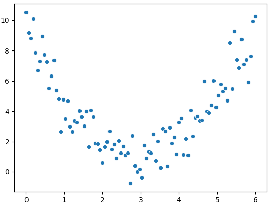
$$r = 0.18$$
Non-linear relationships
What we see:
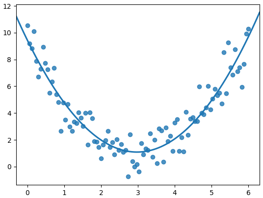
What the correlation coefficient sees:
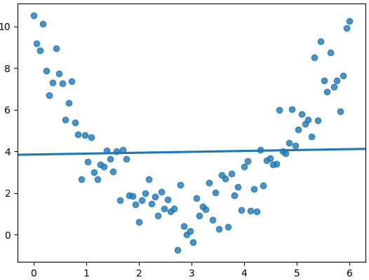
Correlation only accounts for linear relationships
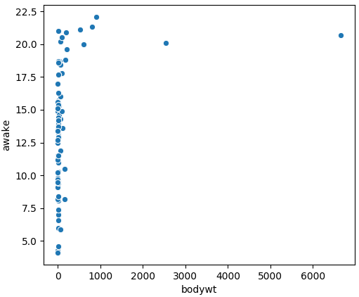
Always visualize your data
Body weight vs. awake time
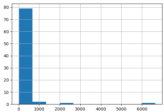
Distribution of body weight
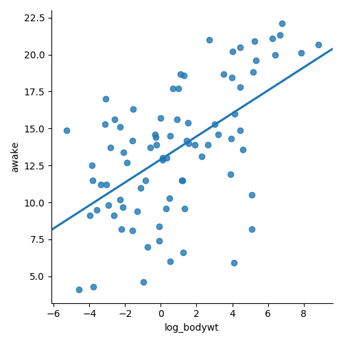
Log transformation
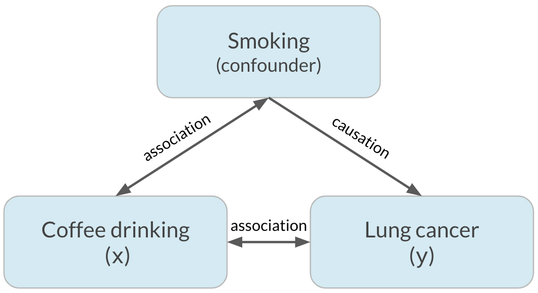
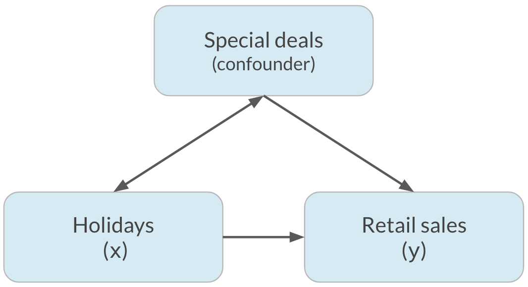
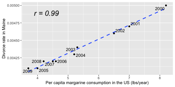
Correlation does not imply causation
x is correlated with y does not mean x causes y
Confounding
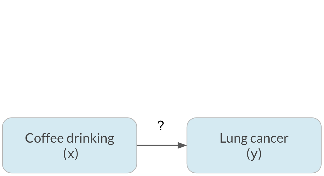
Confounding
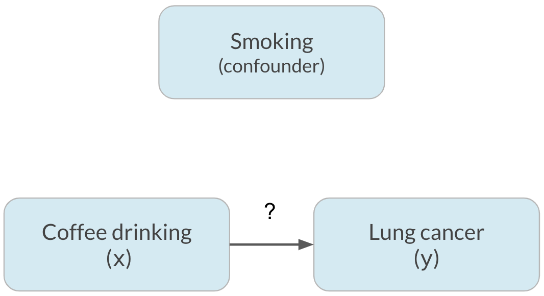
Confounding
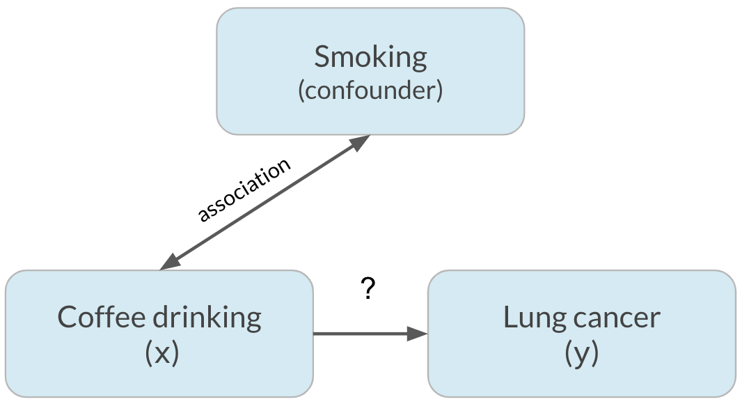
Confounding
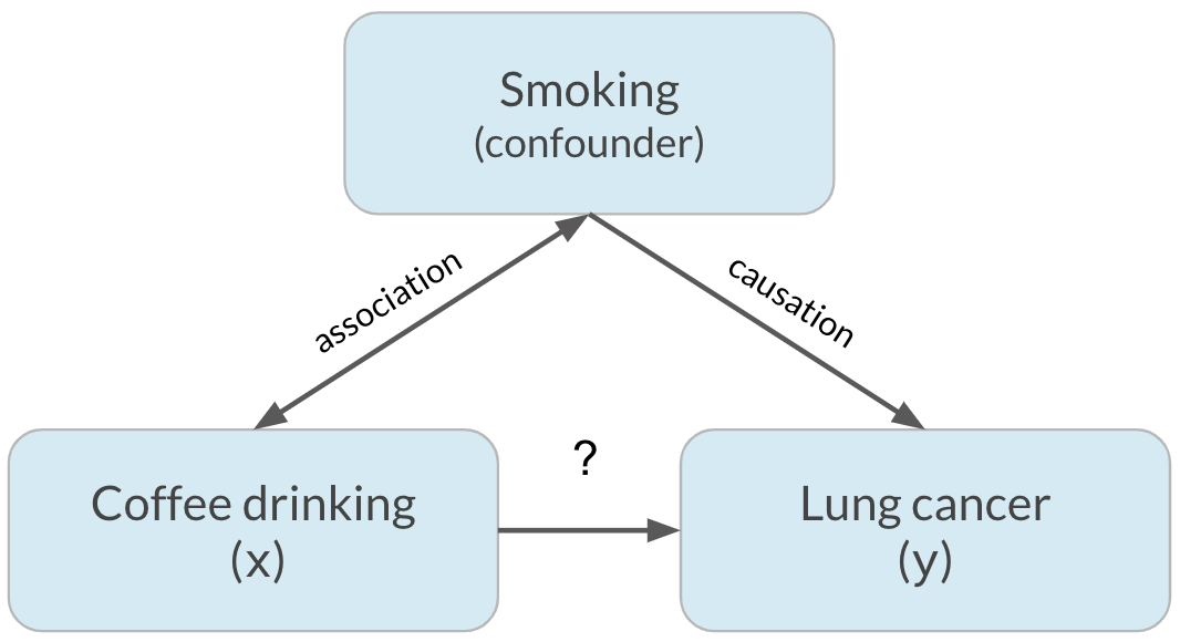
Confounding