Prior belief
Bayesian Data Analysis in Python

Michal Oleszak
Machine Learning Engineer
Prior's impact
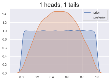
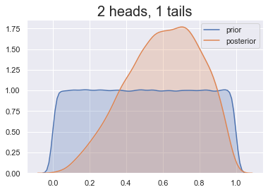
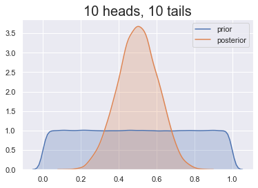
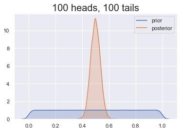
Choosing the right prior
Our prior belief: heads less likely
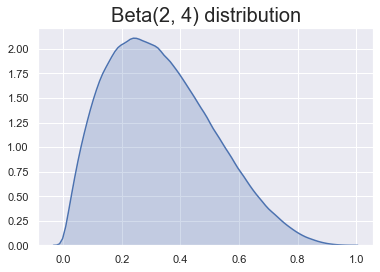
Some choices are better than others!
Bayesian Data Analysis in Python
Michal Oleszak
Machine Learning Engineer
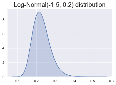
Our prior belief: heads less likely
Some choices are better than others!

