Interpreting results and comparing models

Bayesian Data Analysis in Python

Michal Oleszak

Machine Learning Engineer

Running the model revisited

formula = "num_clicks ~ clothes_banners_shown + sneakers_banners_shown"

with pm.Model() as model_1:
    pm.GLM.from_formula(formula, data=ads_aggregated)
    trace_1 = pm.sample(draws=1000, tune=500)

Running the model revisited

formula = "num_clicks ~ clothes_banners_shown + sneakers_banners_shown"

with pm.Model() as model_1:
    pm.GLM.from_formula(formula, data=ads_aggregated)
    trace_1 = pm.sample(draws=1000, tune=500, chains=4)

Number of parameters: 4
Number of draws for each parameter: 1000 $\times$ 4 = 4000

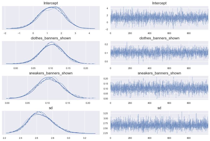
Trace plot

pm.traceplot(trace_1)

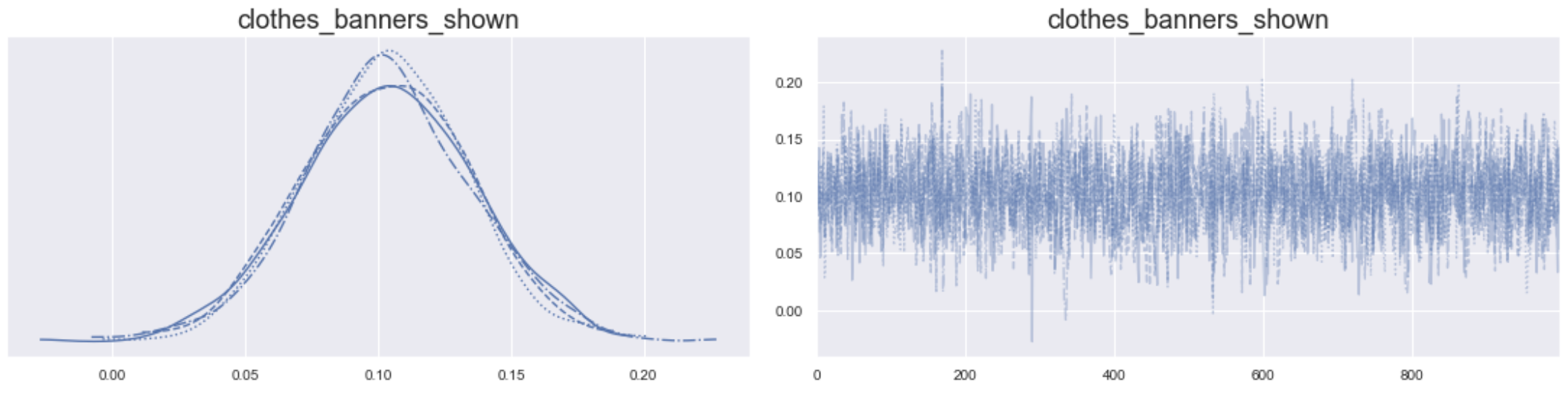
A grid of eight plots in two columns and four rows. The left column contains four density plots, and the right column contains four line plots, each for one model parameter.

Trace plot: zoom in on one parameter

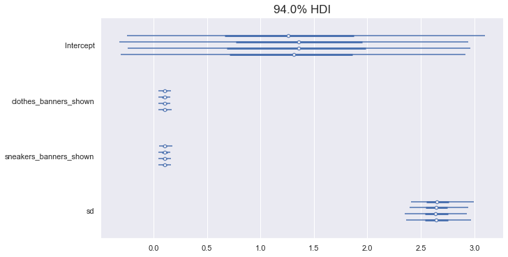
Two plots next to each other: the left one shows a density plot, and the right one a line plot of parameter draws.

Forest plot

pm.forestplot(trace_1)

A plot showing the distribution of draws for each model parameter depicted as a horizontal.

Trace summary

pm.summary(trace_1)

                         mean     sd  hdi_3%  hdi_97%  mcse_mean  mcse_sd  \
Intercept               1.307  0.886  -0.305    2.962      0.018    0.013   
clothes_banners_shown   0.103  0.031   0.043    0.160      0.001    0.000   
sneakers_banners_shown  0.104  0.032   0.045    0.163      0.001    0.001   
sd                      2.654  0.157   2.382    2.970      0.003    0.002   

                        ess_mean  ess_sd  ess_bulk  ess_tail  r_hat  
Intercept                 2346.0  2318.0    2351.0    2083.0    1.0  
clothes_banners_shown     2085.0  2085.0    2089.0    1868.0    1.0  
sneakers_banners_shown    2105.0  1953.0    2122.0    1869.0    1.0  
sd                        2615.0  2590.0    2646.0    1834.0    1.0

Fitting another model

formula = "num_clicks ~ clothes_banners_shown + sneakers_banners_shown + weekend"

with pm.Model() as model_2:
    pm.GLM.from_formula(formula, data=ads_aggregated)
    trace_2 = pm.sample(draws=1000, tune=500)

Widely Applicable Information Criterion (WAIC)

comparison = pm.compare({"trace_1": trace_1, "trace_2": trace_2}, 
                        ic="waic", scale="deviance")
print(comparison)

        rank     waic   p_waic    d_waic    weight       se      dse warning  \
trace_2    0   -362.8   5.1576         0  0.513792  9.37269        0    True   
trace_1    1 -362.926  4.13318  0.126236  0.486208  9.48352  1.50682    True   

        waic_scale  
trace_2        log  
trace_1        log

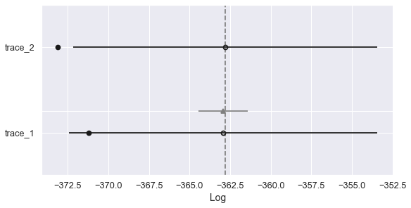
Compare plot

pm.compareplot(comparison)

A plot visualizing the WAIC values for two models.

Let's practice comparing models!

Bayesian Data Analysis in Python