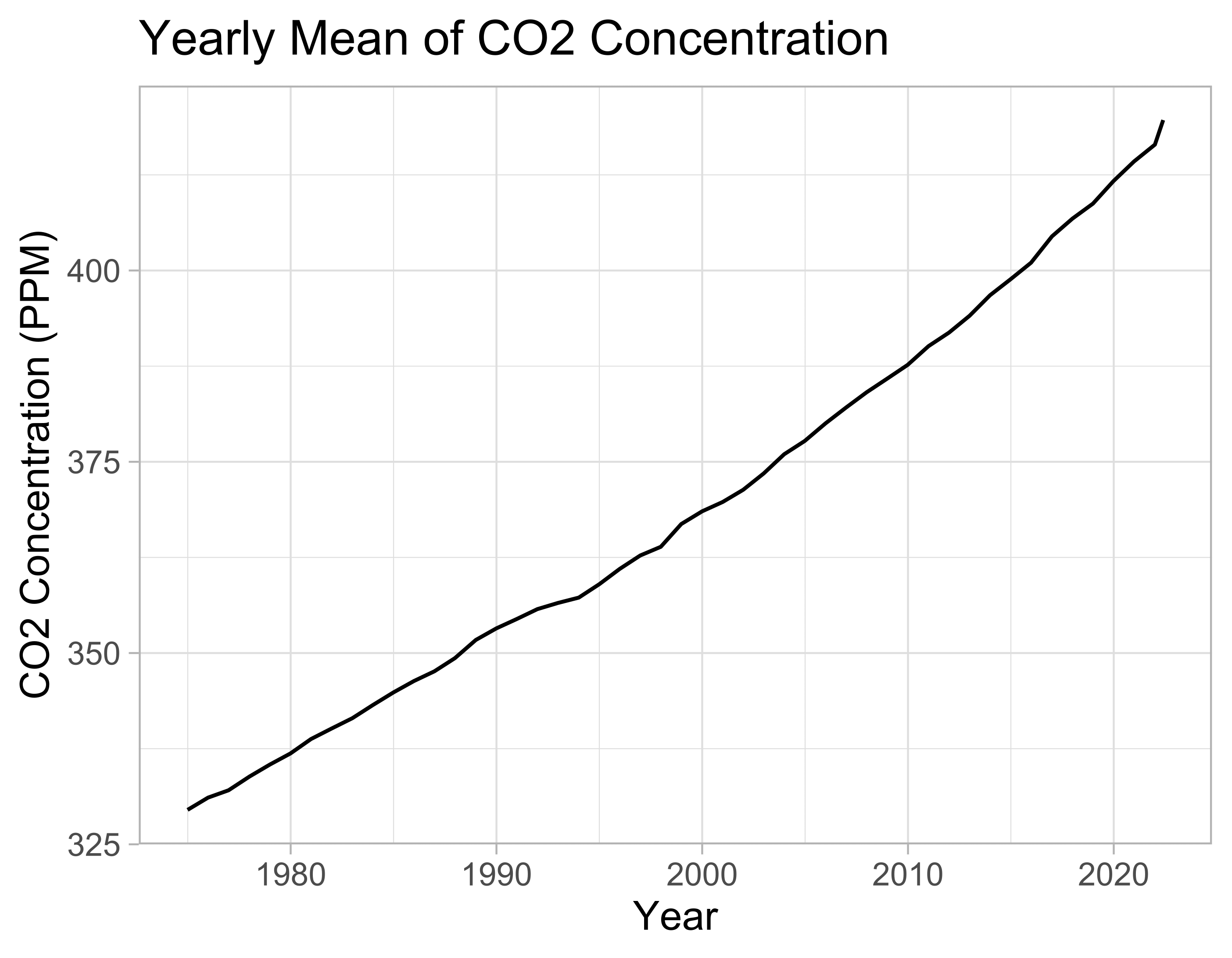
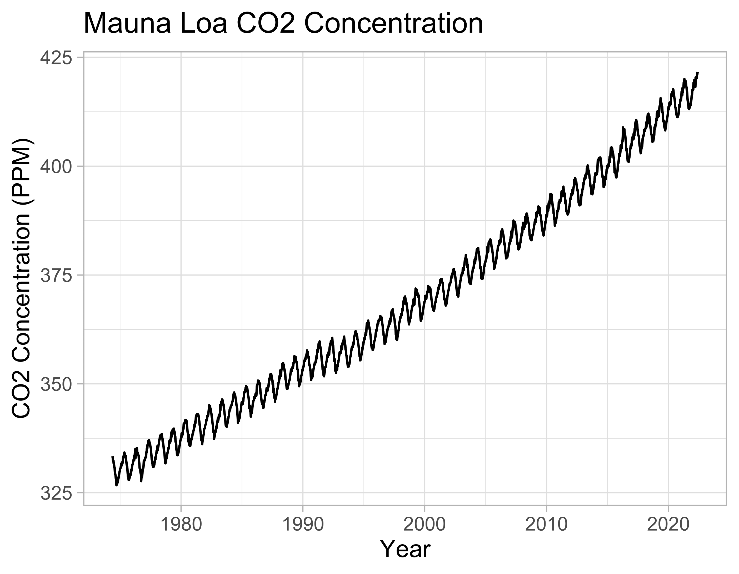
Resampling and aggregating observations

Manipulating Time Series Data in R

Harrison Brown

Graduate Researcher in Geography

Sampling frequency

Frequency:

  • Number of observations per year
  • e.g., weekly, daily, monthly, ...

Temporal resolution:

  • "High resolution" sampled often
  • "Low resolution" sampled infrequently
  • "High" and "low" are subjective

Conceptual diagram showing two grids: one with a low resolution and one with a high resolution. This diagram highlights the idea of data sampled more frequently or less frequently.

Manipulating Time Series Data in R

Aggregation

  • High resolution -> low resolution
  • Applies a function like mean, sum, max to the chosen interval
  • e.g.:
    • Monthly sum of daily data
    • Weekly mean of hourly values
    • ...
  • Cannot 'reverse' aggregation
  • Monthly total -> daily values?
  • Provides statistics to describe patterns in the data
  • Aggregation reduces information
Manipulating Time Series Data in R

Aggregating data with xts

xts:

  • eXtensible Time Series
  • Extends the zoo package and zoo class of objects
  • apply.*() functions
yearly_mean <-
  apply.yearly(x = maunaloa,
               FUN = mean)
autoplot(yearly_mean) + 
  labs(...)

Graph of the Mauna Loa dataset, which has been aggregated to find the yearly average of the data. Rather than in the original data, where there was strong variation within each year, this graph has a very smooth line, as the sampling resolution is much lower.

Manipulating Time Series Data in R

Aggregating data with xts

Graph of the Mauna Loa time series, which represents carbon dioxide concentrations sampled weekly. The graph has a general upwards trend, with a periodic, seasonal peak each year.

Graph of the Mauna Loa dataset, which has been aggregated to find the yearly average of the data. Rather than in the original data, where there was strong variation within each year, this graph has a very smooth line, as the sampling resolution is much lower.

Manipulating Time Series Data in R

apply-dot functions

daily_total <-
  apply.daily(hourly_sales,
              FUN = sum)
weekly_max <-
  apply.weekly(daily_temperature,
               FUN = max)
monthly_average <-
  apply.monthly(daily_price,
               FUN = mean)
apply.quarterly(sales_report,
                FUN = sum)
apply.yearly(monthly_salary,
             FUN = sum)
Manipulating Time Series Data in R

Endpoints and period.apply

xts::endpoints()

xts::period.apply()

biweekly_eps <-
  endpoints(x = daily_data,
            on = "weeks",
            k = 2)
biweekly_data <-
  period.apply(x = daily_data,
               INDEX = biweekly_eps,
               FUN = mean)
biweekly_data
2002-05-05 8.148611
2002-05-19 8.146776
2002-06-02 8.060020
2002-06-16 8.028224
2002-06-30 7.944792
2002-07-14 7.930159
...
Manipulating Time Series Data in R

Let's practice!

Manipulating Time Series Data in R

Preparing Video For Download...