Dynamic regression
Forecasting in R

Rob J. Hyndman
Professor of Statistics at Monash University
US personal consumption and income
autoplot(uschange[,1:2], facets = TRUE) +
  xlab("Year") + ylab("") +
  ggtitle("Quarterly changes in US consumption
          and personal income")
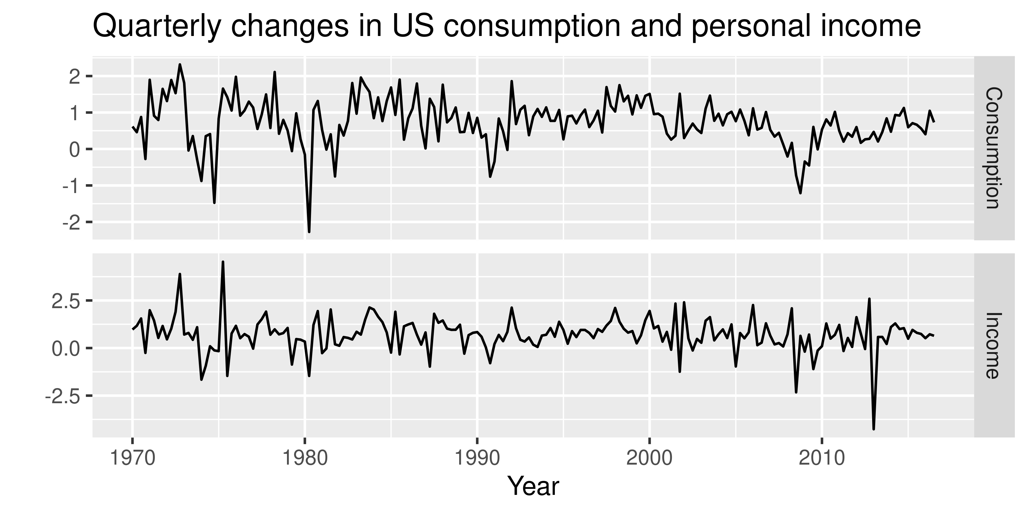
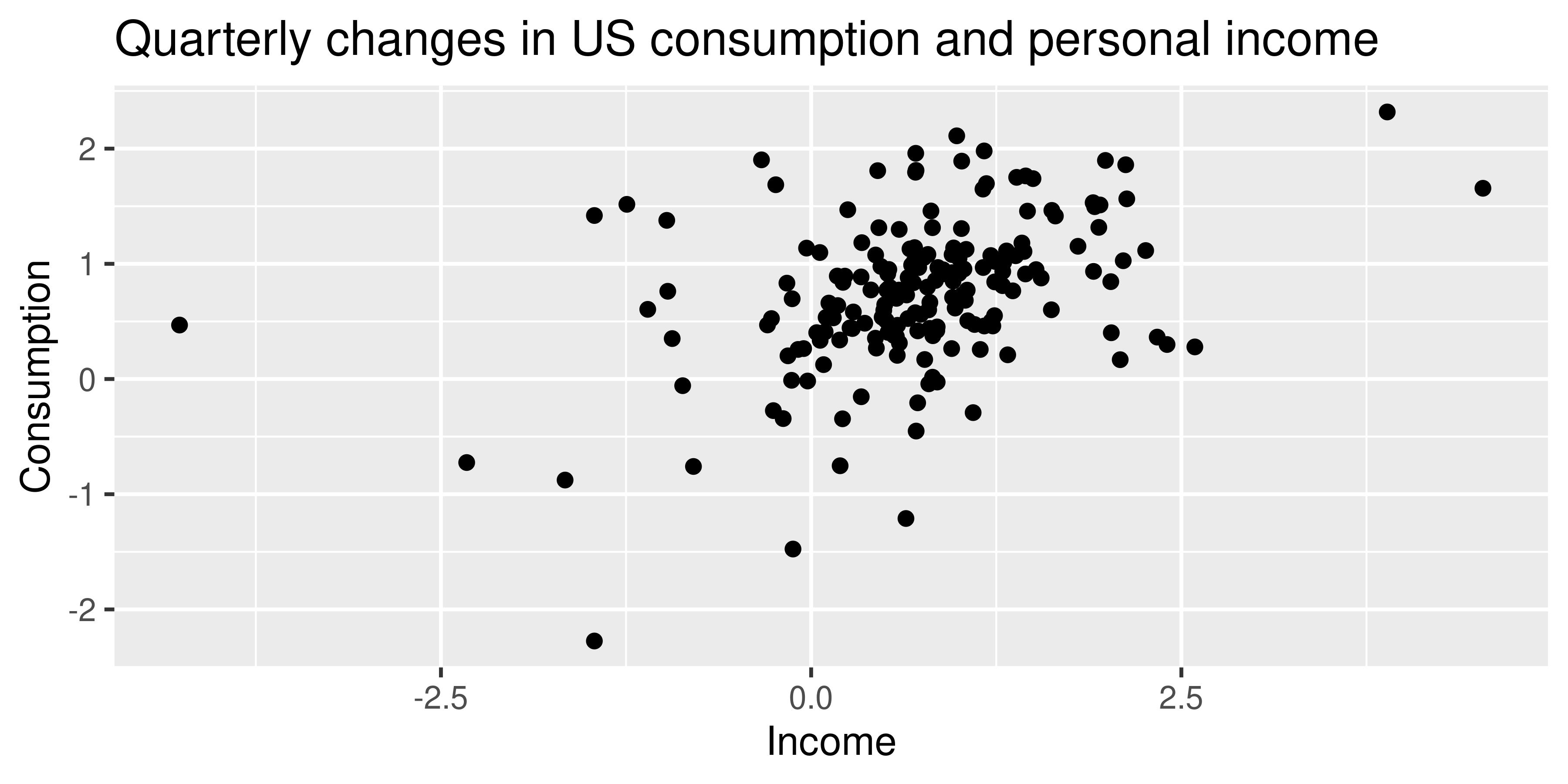
US personal consumption and income
ggplot(aes(x = Income, y = Consumption),
           data = as.data.frame(uschange)) +
  geom_point() +
  ggtitle("Quarterly changes in US consumption and
          personal income")
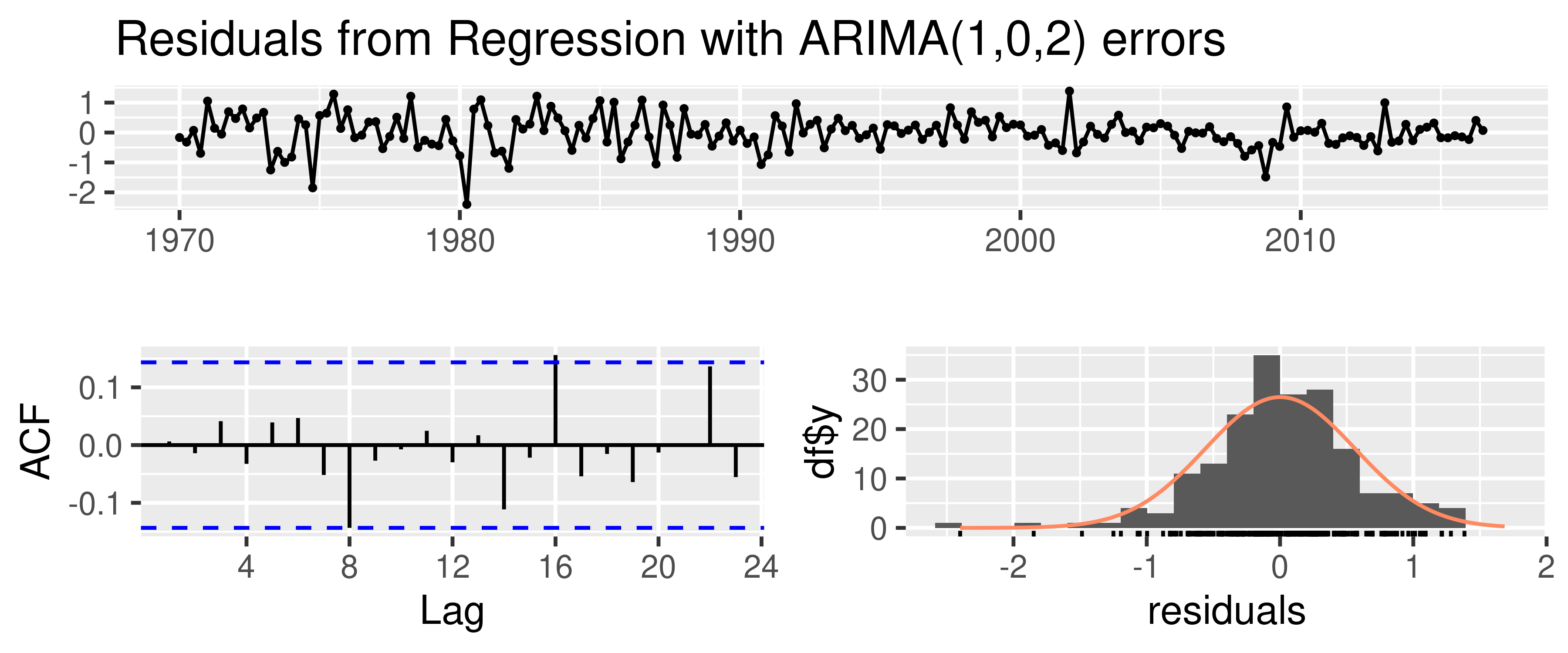
Residuals from dynamic regression model
checkresiduals(fit)
Ljung-Box test
data:  Residuals from Regression with ARIMA(1,0,2) errors
Q* = 5.8916, df = 5, p-value = 0.3169
Model df: 3.   Total lags used: 8
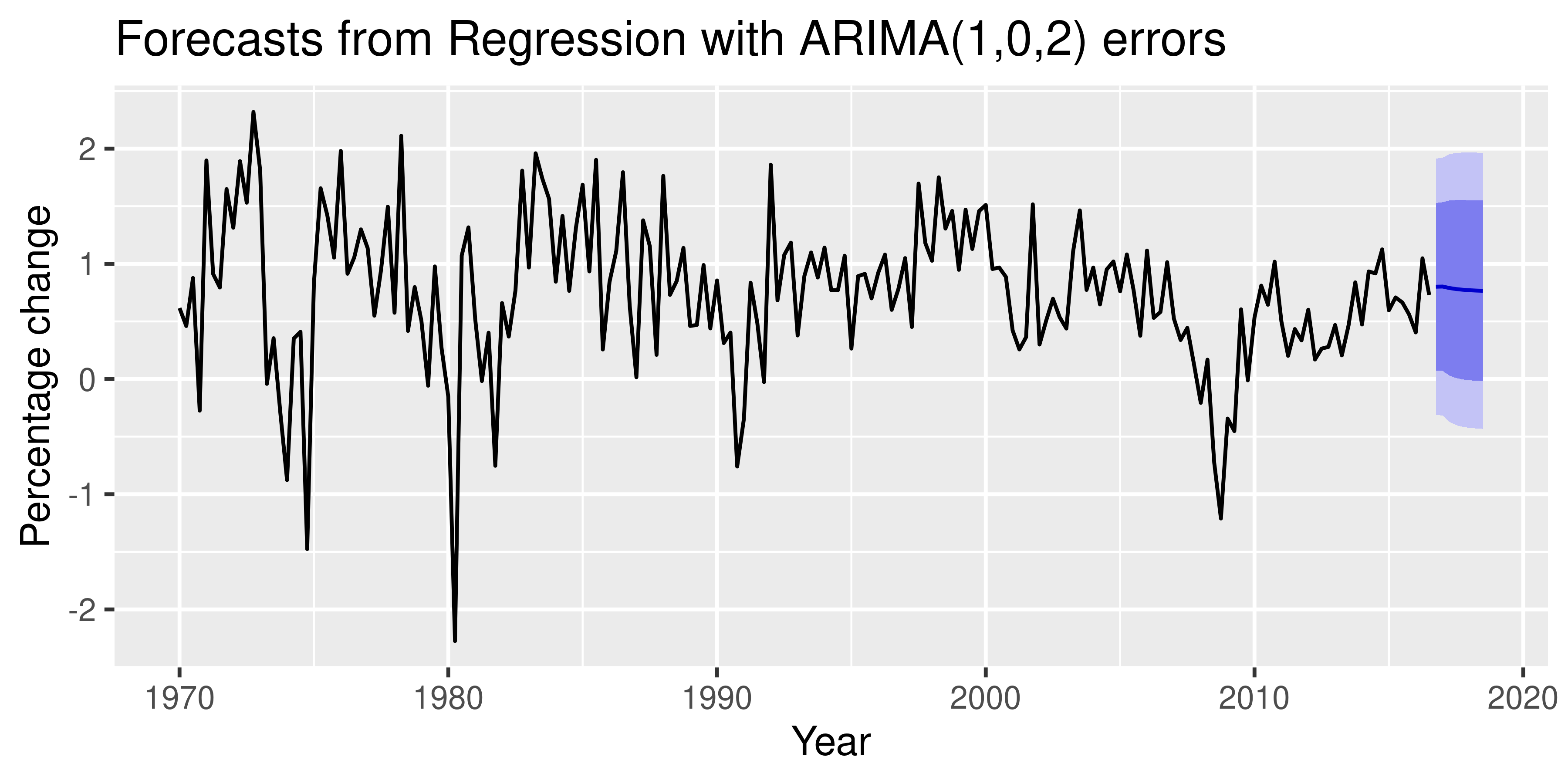
Forecasts from dynamic regression model
fcast <- forecast(fit, xreg = rep(0.8, 8))
autoplot(fcast) +
  xlab("Year") + ylab("Percentage change")