ARIMA models

Forecasting in R

Rob J. Hyndman

Professor of Statistics at Monash University

ARIMA models

Autoregressive (AR) models:

Multiple regression with lagged observations as predictors
$y_t = c + \phi_1 y_{t-1} + \phi_2 y_{t-2} + ... + \phi_p y_{t-p} + e_t$

Moving average (MA) models:

Multiple regression with lagged errors as predictors
$y_t = c + \theta_1 e_{t-1} + \theta_2 e_{t-2} + ... + \theta_q e_{t-q}$

ARIMA models

Autoregressive moving average (ARMA) models:

Multiple regression with lagged observations and errors as predictors
$y_t = c + \phi_1 y_{t-1} + ... + \phi_p y_{t-p} + \theta_1 e_{t-1} + ... + \theta_q e_{t-q} + e_t$

ARIMA(p, d, q) models:

Combine ARMA model with d - lots of differencing

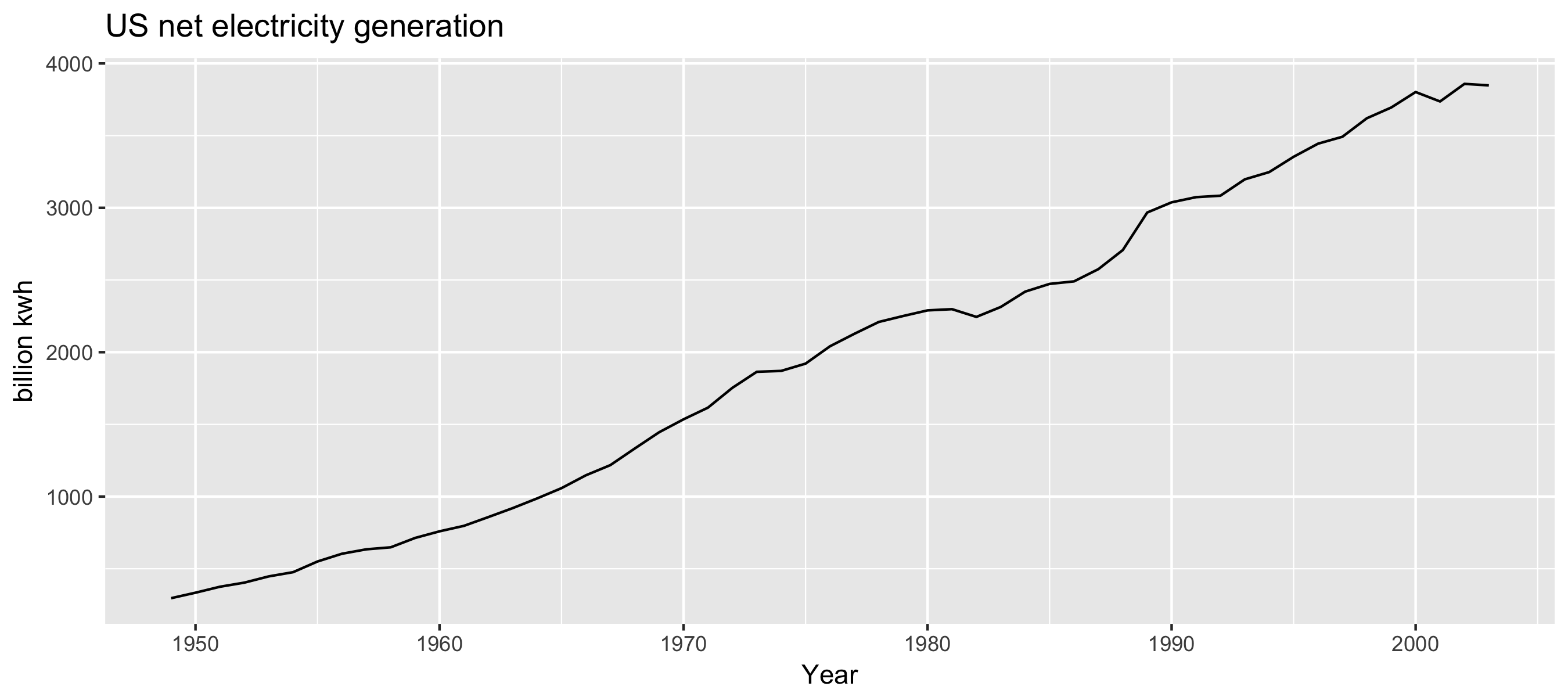
US net electricity generation

autoplot(usnetelec) +
  xlab("Year") +
  ylab("billion kwh") +
  ggtitle("US net electricity generation")

US net electricity generation

fit <- auto.arima(usnetelec)
summary(fit)

Series: usnetelec
ARIMA(2,1,2) with drift
Coefficients:
         ar1     ar2    ma1    ma2   drift
      -1.303  -0.433  1.528  0.834  66.159
s.e.   0.212   0.208  0.142  0.119   7.559
sigma^2 estimated as 2262:  log likelihood=-283.3
AIC=578.7   AICc=580.5   BIC=590.6
Training set error measures:
                 ME  RMSE   MAE     MPE  MAPE   MASE    ACF1
Training set 0.0464 44.89 32.33 -0.6177 2.101 0.4581 0.02249

US net electricity generation

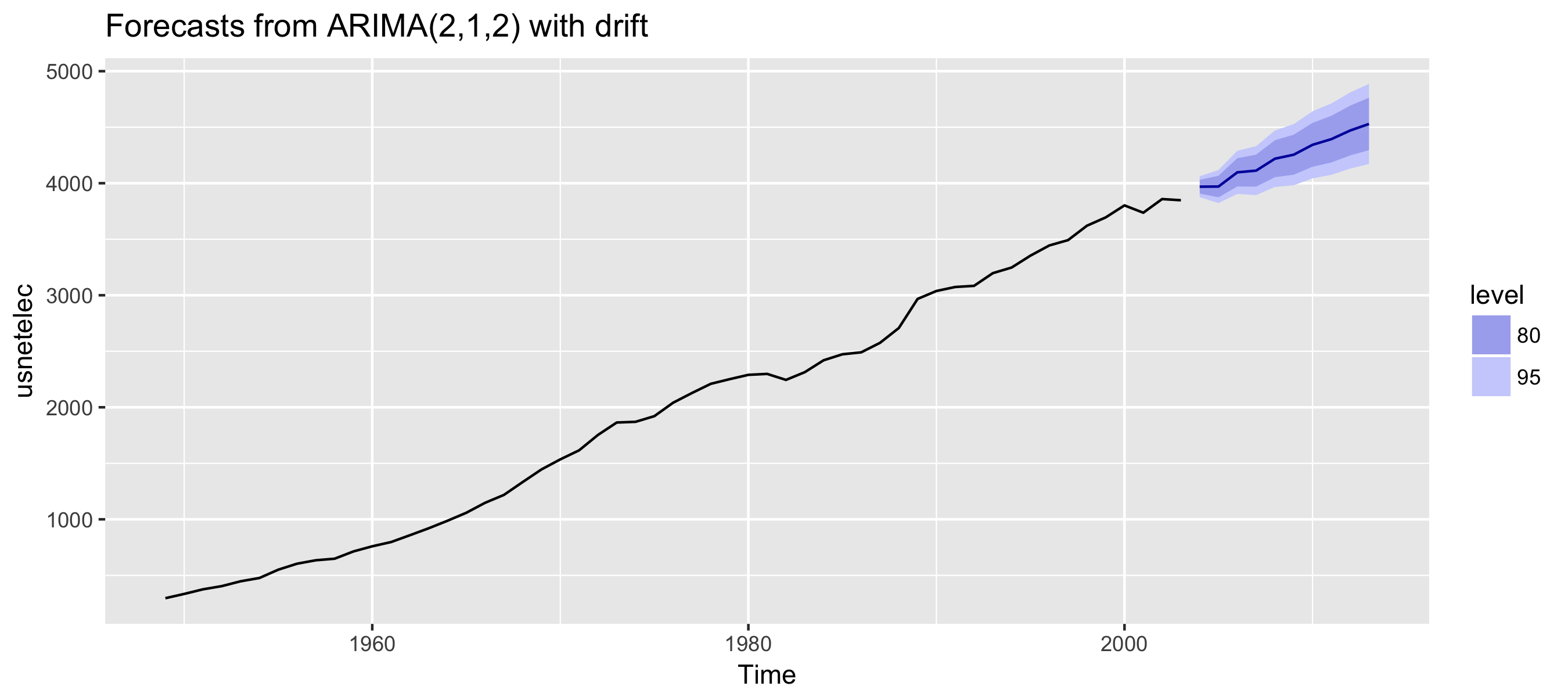
fit %>% forecast() %>% autoplot()

How does auto.arima() work?

Hyndman-Khandakar algorithm:

Select number of differences d via unit root tests
Select p and q by minimizing $AIC_c$
Estimate parameters using maximum likelihood estimation
Use stepwise search to traverse model space, to save time

Let's practice!

Forecasting in R