Dynamic harmonic regression
Forecasting in R

Rob J. Hyndman
Professor of Statistics at Monash University
Dynamic harmonic regression

Dynamic harmonic regression

$m =$ seasonal period
Every periodic function can be approximated by sums of sin and cos terms for large enough K
Regression coefficients: $\alpha_k$ and $\gamma_k$
$e_t$ can be modeled as a non-seasonal ARIMA process
Assumes seasonal pattern is unchanging
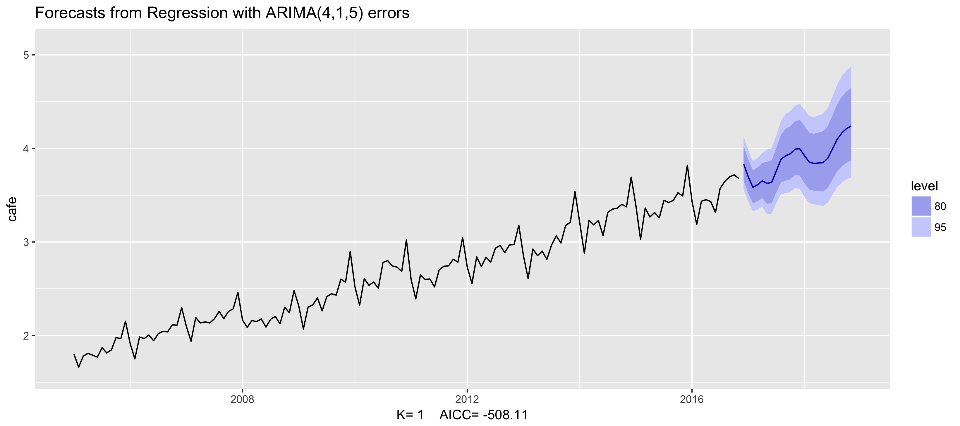
Example: Australian cafe expenditure
fit <- auto.arima(cafe, xreg = fourier(cafe, K = 1),
                  seasonal = FALSE, lambda = 0)
fit %>% forecast(xreg = fourier(cafe, K = 1, h = 24)) %>%
   autoplot() + ylim(1.6, 5.1)
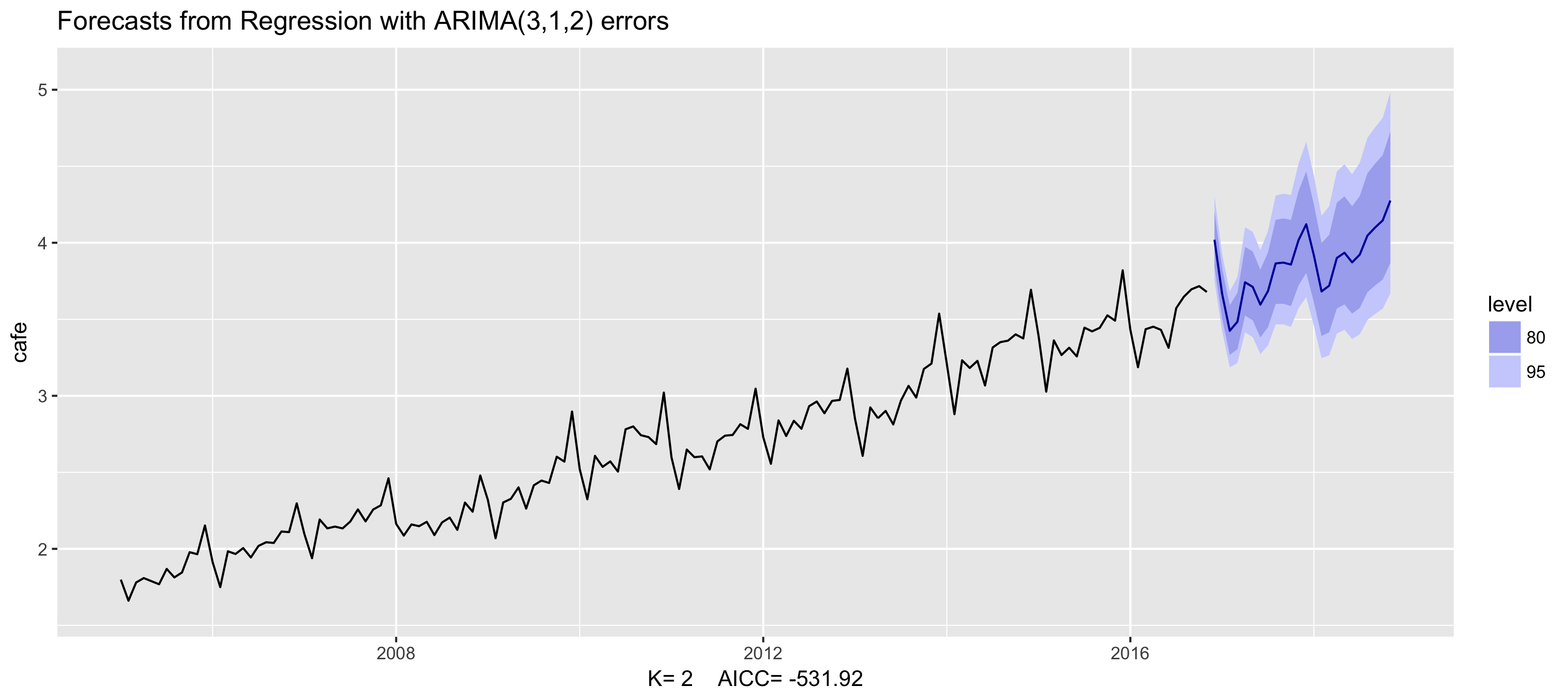
Example: Australian cafe expenditure
fit <- auto.arima(cafe, xreg = fourier(cafe, K = 2),
                  seasonal = FALSE, lambda = 0)
fit %>% forecast(xreg = fourier(cafe, K = 2, h = 24)) %>%
   autoplot() + ylim(1.6, 5.1)
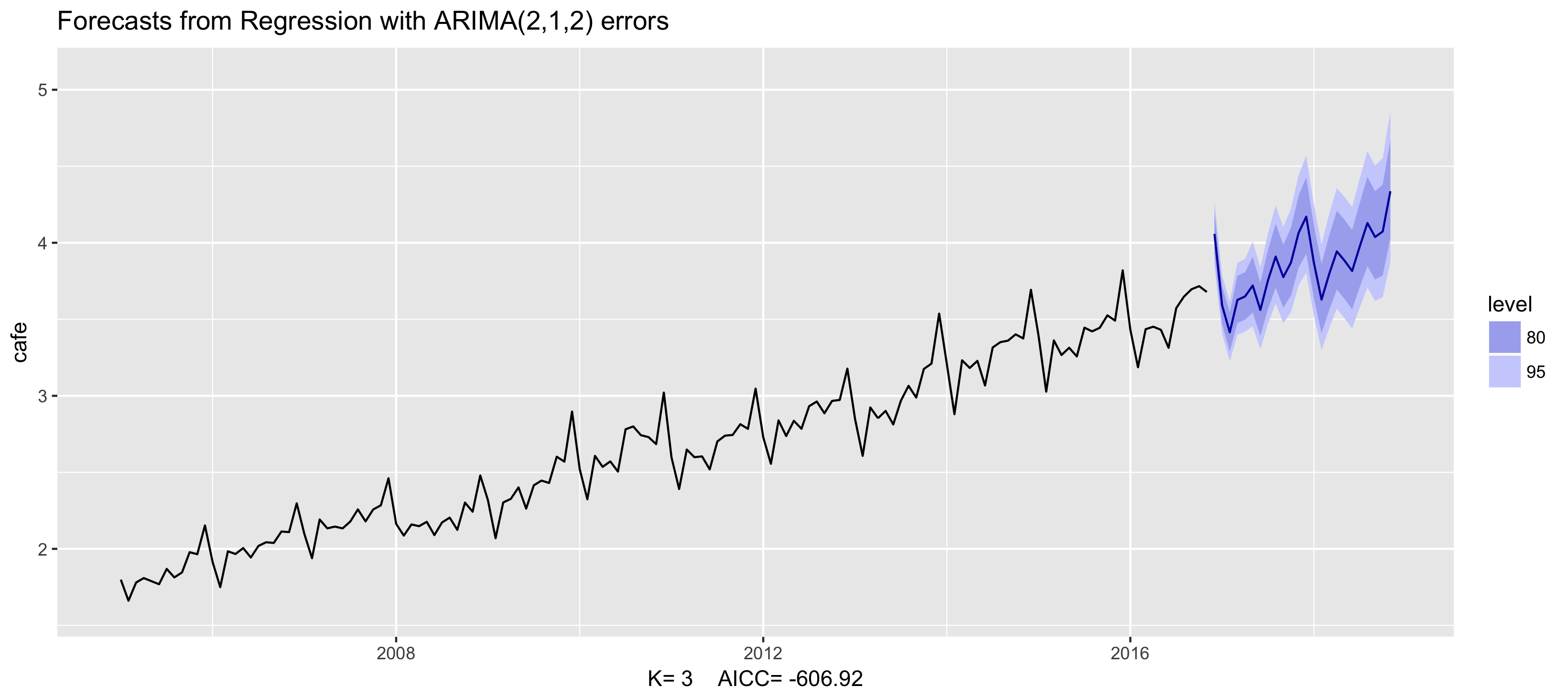
Example: Australian cafe expenditure
fit <- auto.arima(cafe, xreg = fourier(cafe, K = 3),
                  seasonal = FALSE, lambda = 0)
fit %>% forecast(xreg = fourier(cafe, K = 3, h = 24)) %>%
   autoplot() + ylim(1.6, 5.1)
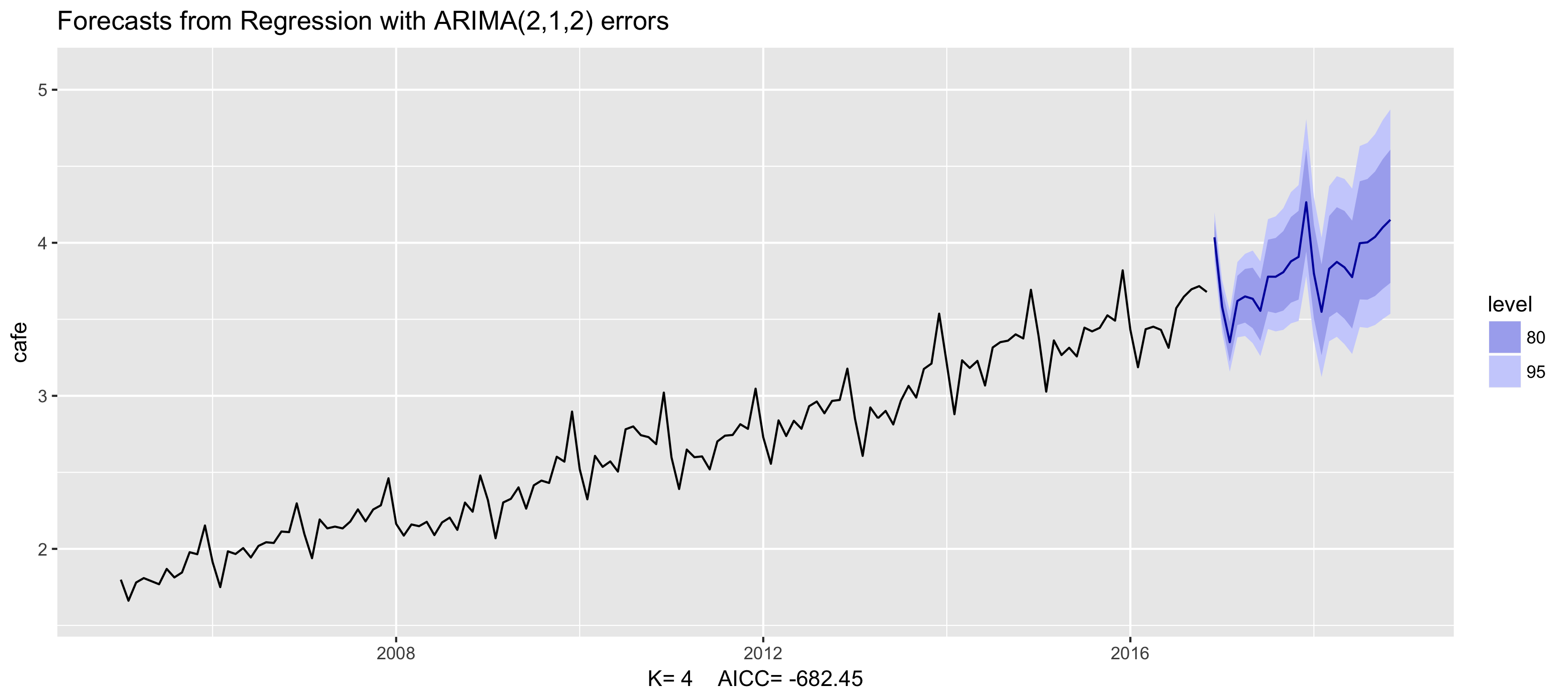
Example: Australian cafe expenditure
fit <- auto.arima(cafe, xreg = fourier(cafe, K = 4),
                  seasonal = FALSE, lambda = 0)
fit %>% forecast(xreg = fourier(cafe, K = 4, h = 24)) %>%
   autoplot() + ylim(1.6, 5.1)
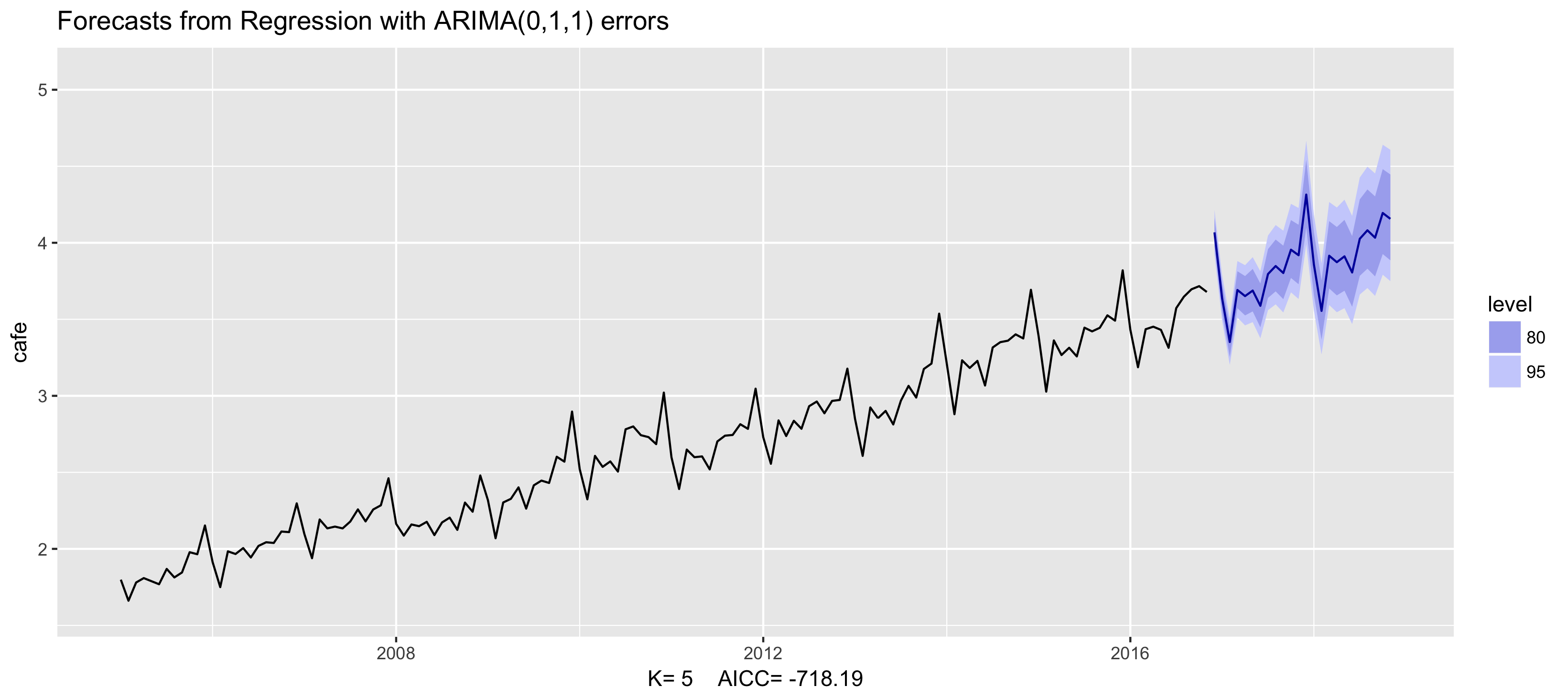
Example: Australian cafe expenditure
fit <- auto.arima(cafe, xreg = fourier(cafe, K = 5),
                  seasonal = FALSE, lambda = 0)
fit %>% forecast(xreg = fourier(cafe, K = 5, h = 24)) %>%
   autoplot() + ylim(1.6, 5.1)
Example: Australian cafe expenditure
fit <- auto.arima(cafe, xreg = fourier(cafe, K = 6),
                  seasonal = FALSE, lambda = 0)
fit %>% forecast(xreg = fourier(cafe, K = 6, h = 24)) %>%
   autoplot() + ylim(1.6, 5.1)

Dynamic harmonic regression

- Other predictor variables can be added as well: $x_{t,1},...,x_{t,r}$
- Choose K to minimize the $AIC_c$
- K can not be more than m/2
- This is particularly useful for weekly data, daily data and sub-daily data.

