Exponentially weighted forecasts
Forecasting in R

Rob J. Hyndman
Professor of Statistics at Monash University
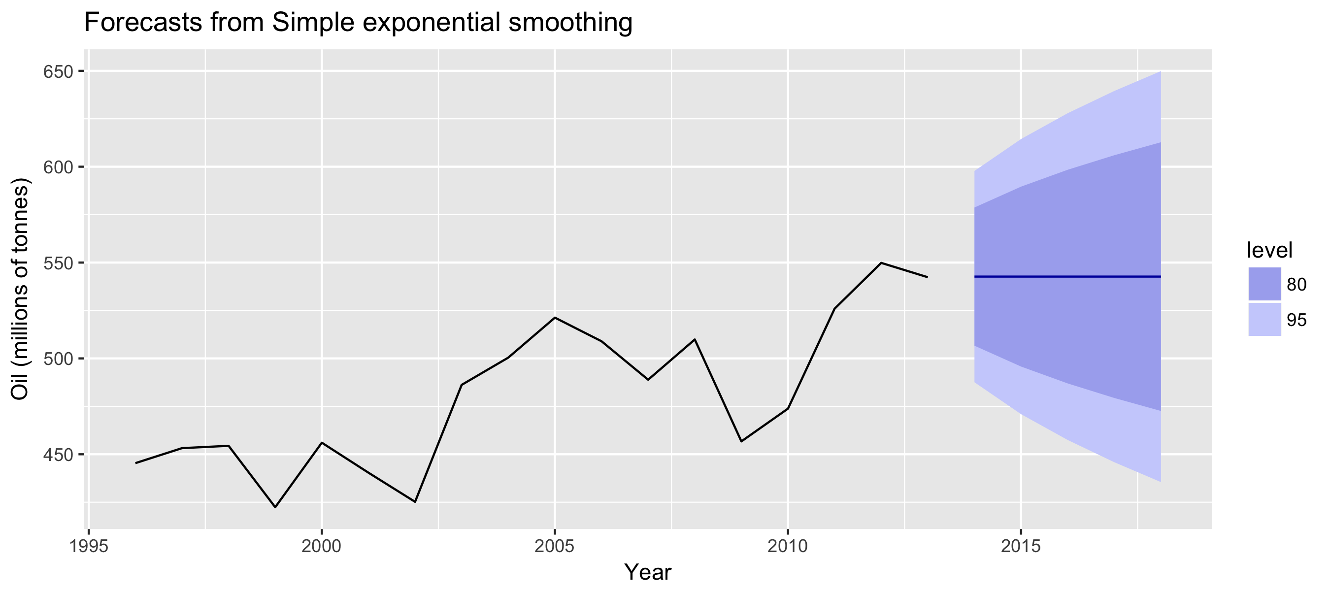
Example: oil production
autoplot(fc) +
  ylab("Oil (millions of tonnes)") + xlab("Year")
Forecasting in R
Rob J. Hyndman
Professor of Statistics at Monash University
autoplot(fc) +
ylab("Oil (millions of tonnes)") + xlab("Year")

