State space models for exponential smoothing
Forecasting in R

Rob J. Hyndman
Professor of Statistics at Monash University
Innovations state space models
- Each exponential smoothing method can be written as an "innovations state space model"

Innovations state space models
- Each exponential smoothing method can be written as an "innovations state space model"

Innovations state space models
- Each exponential smoothing method can be written as an "innovations state space model"

Innovations state space models
- Each exponential smoothing method can be written as an "innovations state space model"

Innovations state space models
- Each exponential smoothing method can be written as an "innovations state space model"

- ETS models: Error, Trend, Seasonal
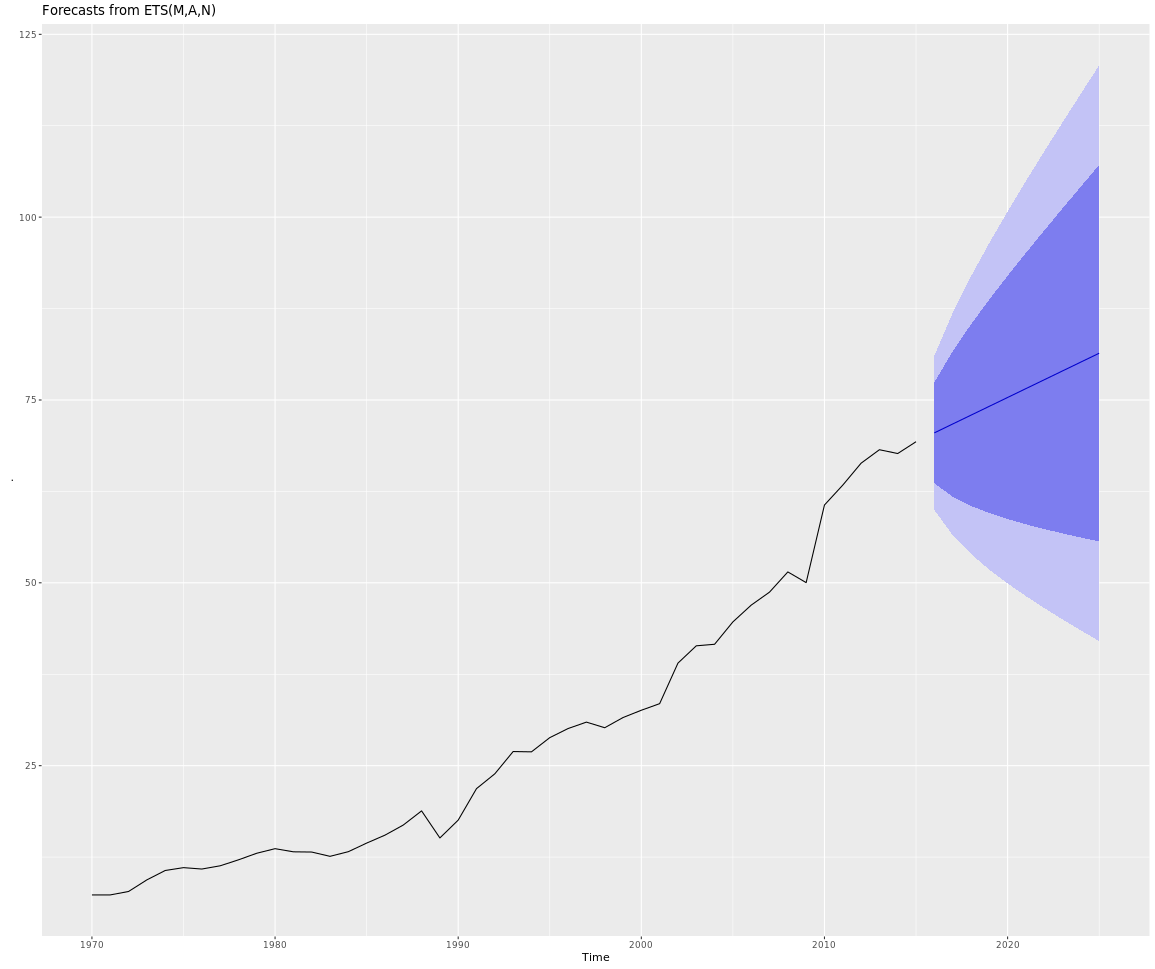
Example: Australian air traffic
ausair %>% ets() %>% forecast() %>% autoplot()
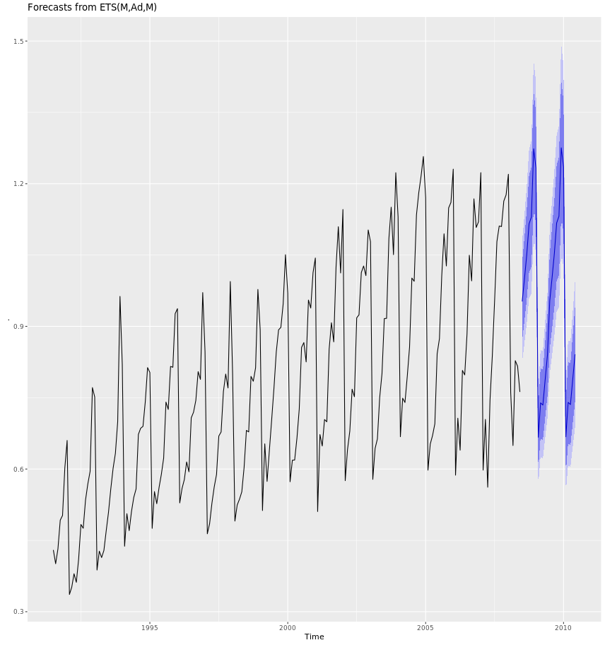
Example: Monthly cortecosteroid drug sales
h02 %>% ets() %>% forecast() %>% autoplot()