Seasonal ARIMA models

Forecasting in R

Rob J. Hyndman

Professor of Statistics at Monash University

ARIMA models

ch4_vid3_slides.003.png

d = Number of lag-1 differences
p = Number of ordinary AR lags:
q = Number of ordinary MA lags:

ARIMA models

ch4_vid3_slides.007.png

d = Number of lag-1 differences
p = Number of ordinary AR lags:
q = Number of ordinary MA lags:

ARIMA models

ch4_vid3_slides.008.png

d = Number of lag-1 differences
p = Number of ordinary AR lags: $\ y_{t-1}, y_{t-2},...,y_{t-p}$
q = Number of ordinary MA lags: $\ \epsilon_{t-1}, \epsilon_{t-2},...,\epsilon_{t-q}$
D = Number of seasonal differences
P = Number of seasonal AR lags: $\ y_{t-m}, y_{t-2m},...,y_{t-Pm}$
Q = Number of seasonal MA lags:$\ \epsilon_{t-m}, \epsilon_{t-2m},...,\epsilon_{t-Qm}$
m = Number of observations per year

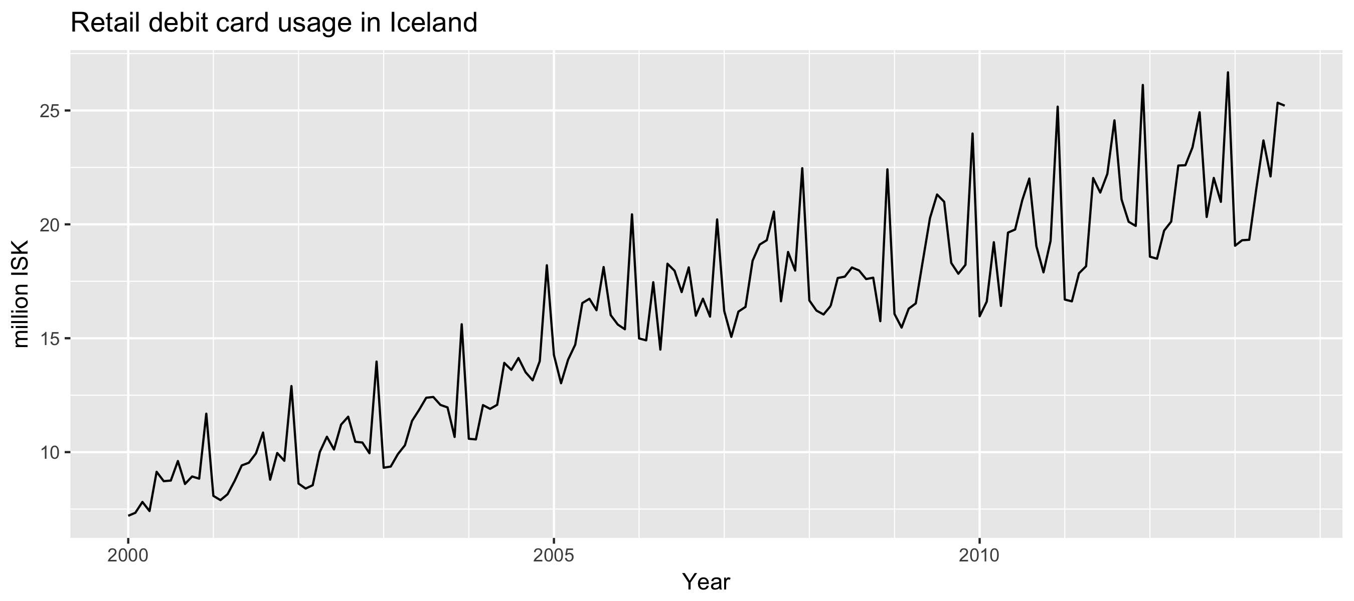
Example: Monthly retail debit card usage in Iceland

autoplot(debitcards) +
  xlab("Year") + ylab("million ISK") +
  ggtitle("Retail debit card usage in Iceland")

Example: Monthly retail debit card usage in Iceland

fit <- auto.arima(debitcards, lambda = 0)
fit

Series: debitcards
ARIMA(0,1,4)(0,1,1)[12]
Box Cox transformation: lambda= 0
Coefficients:
         ma1    ma2    ma3     ma4    sma1
      -0.796  0.086  0.263  -0.175  -0.814
s.e.   0.082  0.099  0.100   0.080   0.112
sigma^2 estimated as 0.00232:  log likelihood=239.3
AIC=-466.7   AICc=-466.1   BIC=-448.6

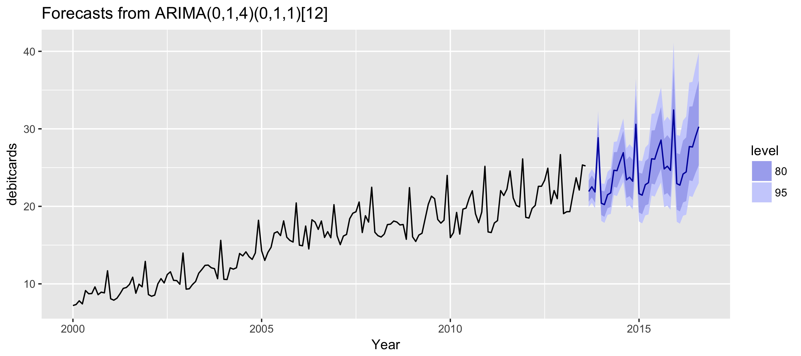
Example: Monthly retail debit card usage in Iceland

fit %>%
  forecast(h = 36) %>%
  autoplot() + xlab("Year")

Let's practice!

Forecasting in R