Exponential smoothing methods with trend and seasonality
Forecasting in R

Rob J. Hyndman
Professor of Statistics at Monash University
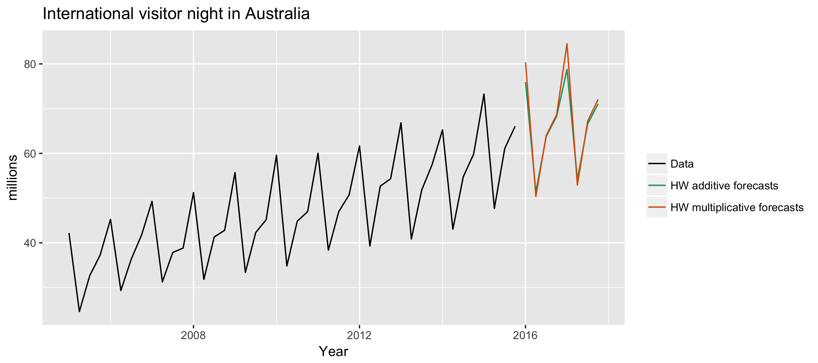
Example: Visitor Nights
aust <- window(austourists, start = 2005)
fc1  <- hw(aust, seasonal = "additive")
fc2  <- hw(aust, seasonal = "multiplicative")
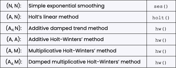
Taxonomy of exponential smoothing methods
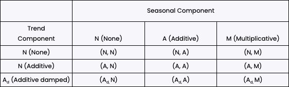
Taxonomy of exponential smoothing methods