Exponential smoothing methods with trend

Forecasting in R

Rob J. Hyndman

Professor of Statistics at Monash University

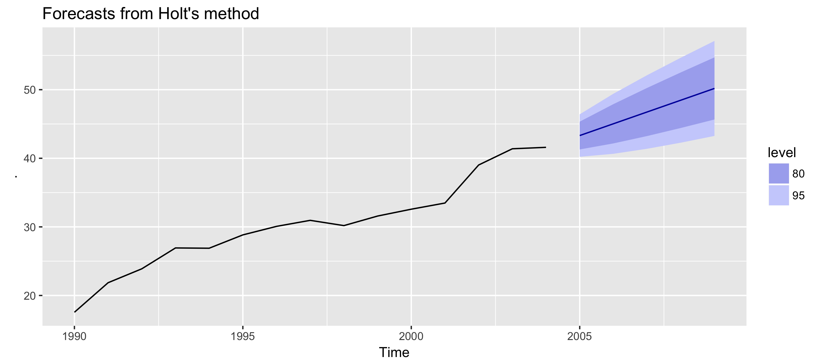
Holt's linear trend

	Simple exponential smoothing
Forecast	$\hat{y}_{t+h \mid t} = \ell_t$
Level	$\ell_t = \alpha y_t + (1-\alpha)\ell_{t-1}$

	Holt's linear trend
Forecast	$\hat{y}_{t+h \mid t} = \ell_t + hb_t$
Level	$\ell_t = \alpha y_t + (1-\alpha)(\ell_{t-1} + b_{t-1})$
Trend	$b_t = \beta^(\ell_t = \ell_{t-1}) + (1 - \beta^) b_{t-1}$

Holt's linear trend

	Holt's linear trend
Forecast	$\hat{y}_{t+h \mid t} = \ell_t + hb_t$
Level	$\ell_t = \alpha y_t + (1-\alpha)(\ell_{t-1} + b_{t-1})$
Trend	$b_t = \beta^(\ell_t = \ell_{t-1}) + (1 - \beta^) b_{t-1}$

Two smoothing parameters $\alpha$ and $\beta^*$ where $0 \leq \alpha$ and $\beta^* \leq 1$
Choose $\alpha, \beta^*, \ell_0, b_0$ to minimize SSE

Holt's method in R

airpassengers %>% holt(h = 5) %>% autoplot

Damped trend method

Component form
$\hat{y}_{t+h \mid t} = \ell_t + (\phi + \phi^2 + ... + \phi^h)b_t$
$\ell_t = \alpha y_t + (1-\alpha)(\ell_{t-1} + \phi b_{t-1})$
$b_t = \beta^(\ell_t = \ell_{t-1}) + (1 - \beta^) \phi b_{t-1}$

Damping parameter $\ 0 < \phi < 1$
If $\ \phi = 1$, identical to Holt's linear trend
Short-run forecasts trended, long-run forecasts constant

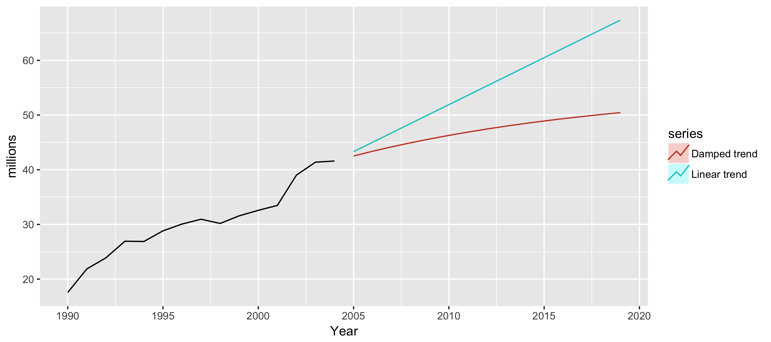
Example: air passengers

fc1 <- holt(airpassengers, h = 15, PI = FALSE)
fc2 <- holt(airpassengers, damped = TRUE, h = 15, PI = FALSE)
autoplot(airpassengers) + xlab("Year") + ylab("millions") +
  autolayer(fc1, series="Linear trend") +
  autolayer(fc2, series="Damped trend")

Let's practice!

Forecasting in R