Basics of time series data transformation

Time Series Analysis in Power BI

Kevin Barlow

Data Analytics Professional

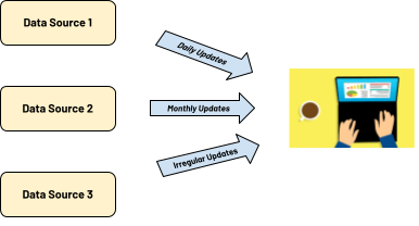
Context and importance

Time series data has become increasingly prevalent in every industry.
Different systems have different requirements and formats.

Mockup Data Architecture

ISO as the international standard

ISO 8601

An international standard for managing date and time data
Allows for translation of dates and times into different formats
Provides localization and personalization for individual needs
Manipulate your date field with FORMAT()

Example Date:

var date = January 1st 2022 
# US Standard (MM DD YYYY)

var date2 = FORMAT(date, "DD MM YYYY")
# UK Standard
# 1 January 2022

var date3 = FORMAT(date, "YYYY MM DD")
# ISO Standard
# 2022 January 01

¹ https://en.wikipedia.org/wiki/ISO_8601#Combined_date_and_time_representations

UNIX for high-precision timestamps

UNIX Time

Also referred to as Epoch time
Signified the number of seconds that have passed since the Epoch time (January 1st, 1970, at 00:00:00 UTC)
UNIX time typically applies to computer systems
Represents a timestamp (date and time)

Example dates and times

January 1st, 2022 06:00:00 UTC

1641016800

January 1st, 2022 18:00:00 UTC

1641060000

¹ https://en.wikipedia.org/wiki/Unix_time

Manipulating dates in Power BI

DATEADD()

Allows you to move a specified number of time intervals from a reference date.

DATEADD(<dates>,<number_of_intervals>,<interval>)

Examples:

DATEADD('date', 30, DAY)

var timestamp_PST = 
    DATEADD('timestamp_EST', -3, HOUR)

DATEDIFF()

Calculates the number of time intervals between two date objects.

DATEDIFF(<Date1>, <Date2>, <Interval>)

Examples:

DATEDIFF(DATE(2019,2,1),
        DATE(2020,4,30),
        MONTH)

Result: 14

Summarizing data with DAX

Time Series does not always come in regular intervals, and depends on how the data is collected. This can be problematic:

Time algorithms and equations assume a consistent interval
Significant changes can happen in between data points

SUMMARIZE() your table to "smooth" out the dataset. By aggregating our dataset, we can still get valuable information on trends, even if data is missing or irregular.

Example:

SUMMARIZE('<table>', 
    [group_column(s)], 
    [new aggregated column(s)])

SUMMARIZE('sales', 
    sales[Quarter], 
    sales[Region], 
    "Total Sales", SUM(sales[revenue]))

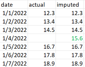
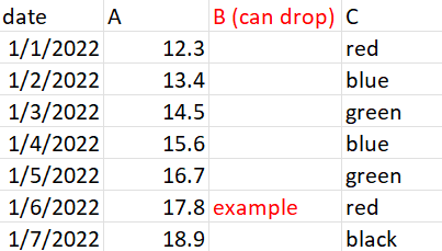
Handling missing data

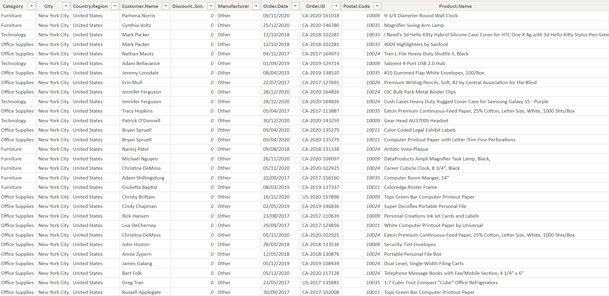
Imputation - a useful strategy when we have lots of context about what the missing data value should be; this is often done when in Power Query.

Imputing Data Example

Dropping data - can be used when a row or column is missing significant amounts of data; should be avoided unless strongly benefits our analysis

Dropping Data Example

Superstore dataset

In the following exercises, you will be looking at the Superstore dataset. This dataset represents Point of Sale (PoS) data for Superstore locations across the United States. With it, you will be formatting dates to a correct format for further analysis.

Superstore Data

Let's practice!

Time Series Analysis in Power BI