Visualizing ratios for within-company analysis

Analyzing Financial Statements in Python

Rohan Chatterjee

Risk modeler

Visualizing financial ratios

Bar plots are helpful for
- visualizing financial ratios for a company on average, and
- assessing performance relative to the industry average

This is an image of a bar plot where we compare the financial ratios of Google with the average of those ratios in the tech industry.

Preparing data for plotting

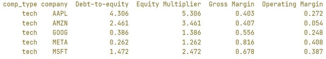
Using pivot_table to compute the average of the ratios by company:

avg_company_ratio = plot_dat.pivot_table(index=["comp_type",
                                                "company"],
                      values=["Gross Margin", "Operating Margin",
                              "Debt-to-equity", "Equity Multiplier"],
                                        aggfunc="mean").reset_index()

print(avg_company_ratio.head())

This image shows the top five rows of the DataFrame avg_company_ratio. The columns of interest here are the gross and operating margin columns. These columns show the average of those ratios for various companies.

Preparing data for plotting

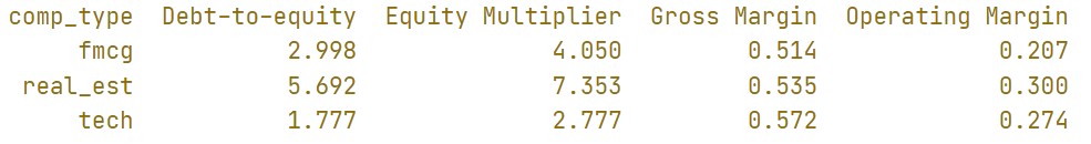
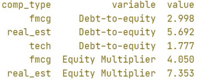
Use pivot_table to compute the average ratio by industry:

avg_industry_ratio = plot_dat.pivot_table(index="comp_type",
                      values=["Gross Margin", "Operating Margin",
                              "Debt-to-equity", 
                              "Equity Multiplier"],
                                        aggfunc="mean").reset_index()

print(avg_industry_ratio.head())

This image shows the top five rows of the DataFrame avg_industry_ratio. The columns of interest here are the gross and operating margin columns. These columns show the average of those ratios for various industries.

Preparing data for plotting

Plotting data in seaborn requires the data to be in a "long" format. Use pd.melt to melt the DataFrames avg_industry_ratio and avg_company_ratio into long format:

molten_plot_company = pd.melt(avg_company_ratio, id_vars=["comp_type",
                                                          "company"])
molten_plot_industry = pd.melt(avg_industry_ratio,
                               id_vars=["comp_type"])

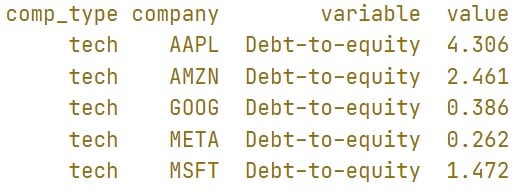
print(molten_plot_company.head())

This image here shows the top 5 rows of the DataFrame molten_plot_industry. The main thing to see here is how the DataFrame is now is the long format of the DataFrame average_industry_ratio. The column variable tells us the name of the ratio and the column value gives us the value of the said ratio.

print(molten_plot_industry.head())

This image here shows the top 5 rows of the DataFrame molten_plot_industry. The main thing to see here is how the DataFrame is now is the long format of the DataFrame average_company_ratio. The column variable tells us the name of the ratio and the column value gives us the value of the said ratio.

Preparing data for plotting

Seaborn requires all the data we want to plot in one DataFrame
We use pd.concat to concatenate molten_plot_company and molten_plot_industry
molten_plot_industry does not have the company DataFrame because it contains the average of the ratios per industry overall
pd.concat requires both DataFrames should to have the same columns, so we add the column company to molten_plot_industry

molten_plot_industry["company"] = "Industry Average"
molten_plot = pd.concat([molten_plot_company, molten_plot_industry])

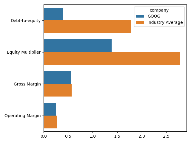
Make the bar graph

sns.barplot(data=molten_plot, y="variable", x="value", hue="company", ci=None)
plt.xlabel(""), plt.ylabel("")
plt.show()

This is the same image as seen in slide 2 of this video. It is an image of a bar plot where we compare the financial ratios of Google with the average of those ratios in the tech industry.

Let's practice!

Analyzing Financial Statements in Python