Geospatial maps with sf

Building Dashboards with shinydashboard

Png Kee Seng

Researcher

An introduction to sf

Use sf to create geospatial maps
- Short for "simple features"
A sf geospatial visualization is always created in layers
- Like layers of masterful brush strokes on a blank canvas
- We shall not delve deeply into the topic of geospatial visualizations

Brush strokes on a blank canvas.

¹ Image by rawpixel.com on Freepik

Importing library and geospatial data

Import sf and tidyverse
Use st_read() and st_as_sf() to read keyhole markup language (KML) files
- london_poly: geospatial boundaries of London
- london_loop: circular (almost) path surrounding London
- london_capital: circular path linking parts of inner London
- listings_geo: coordinates of Airbnb listings

library(sf)
library(tidyverse)

london_poly <- st_read("../data/london_boroughs_boroughs_kml.kml",
                            drivers = "KML", quiet=TRUE)

london_loop <- st_read("../data/London-Loop-SWC-Walk-L24.kml",
                       drivers = "KML", quiet=TRUE)

london_capital <- st_read("../data/Capital-Ring-SWC-Walk-L23.kml",
                          drivers="KML", quiet=TRUE)

listings_geo <- st_as_sf(listings,
                         coords = c("longitude", "latitude"))

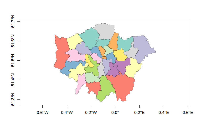
Different types of sf objects: MULTIPOLYGON

london_poly$geometry

Geometry set for 33 features 
Geometry type: MULTIPOLYGON

Dimension:     XY
Bounding box:  xmin: -0.508813 ymin: 51.28691 ...
Geodetic CRS:  WGS 84
First 5 geometries:
MULTIPOLYGON (((-0.183361 51.66868, -0.183383 5...
MULTIPOLYGON (((0.158044 51.50904, 0.156309 51....
MULTIPOLYGON (((-0.212138 51.55558, -0.212689 5...
MULTIPOLYGON (((0.076463 51.431, 0.075932 51.43...
MULTIPOLYGON (((-0.140804 51.56946, -0.14081 51...

Random polygon with 10 sides.

Random polygon with 15 sides.

Different types of sf objects: LINESTRING

london_loop$geometry

Geometry set for 1 feature 
Geometry type: LINESTRING
Dimension:     XYZ
Bounding box:  xmin: -0.499406 ymin: 51.29375 xmax: 0.257656 ymax: 51.67563
z_range:       zmin: 0 zmax: 174
Geodetic CRS:  WGS 84
LINESTRING Z (0.236477 51.48095 1, 0.235149 51....

Same for london_capital

Different types of sf objects: POINT

listings_geo$geometry

Geometry set for 69351 features 
Geometry type: POINT
Dimension:     XY
Bounding box:  xmin: -0.5236 ymin: 51.27248 xmax: 0.30515 ymax: 51.70893
CRS:           NA
First 5 geometries:
POINT (-0.05396 51.52874)
POINT (-0.1127 51.56861)
POINT (-0.07426 51.52851)
POINT (-0.10484 51.52478)
POINT (-0.20004 51.51464)

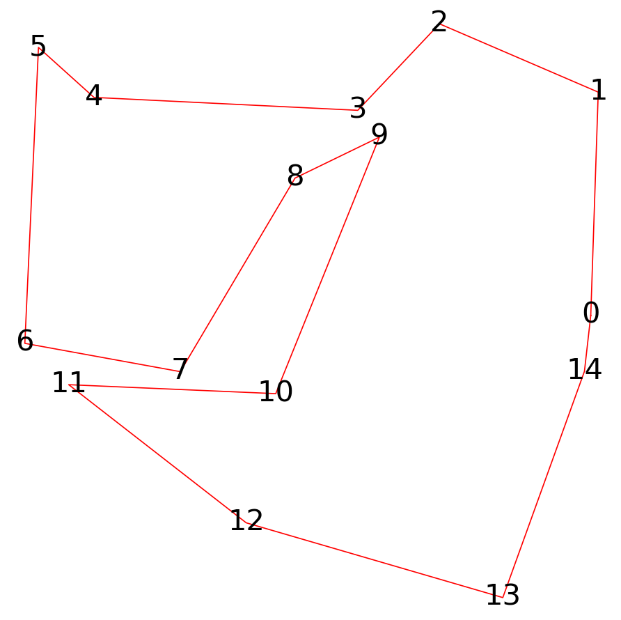
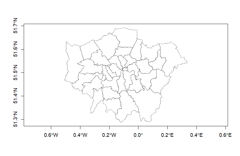
Plotting polygons using plot()

Use st_geometry() to create polygons
Use plot()
Fill each polygon with a different color by setting col

plot(st_geometry(london_poly), axes=TRUE, 
                border=grey(0.2, 0.5))

plot(st_geometry(london_poly), 
        col = sf.colors(length(london_poly$Name), 
                        categorical = TRUE), 
        axes=TRUE, border=grey(0.2, 0.5))

Multi-polygon plots with no color filling.

Multi-polygon plots with color filling.

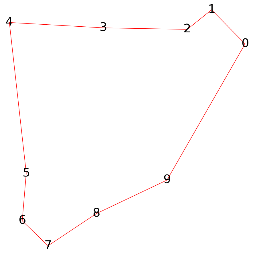
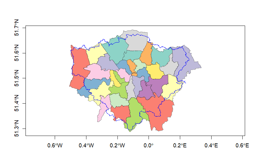
Plotting lines using plot()

Use st_geometry() to create polylines for london_loop
- Set add to TRUE
- Change col to blue
Do the same for london_capital

plot(st_geometry(london_loop),

        add=TRUE,

        col="blue")

plot(st_geometry(london_capital), 
        add=TRUE, 
        col="darkgreen")

Map with one circular path.

Map with two circular paths.

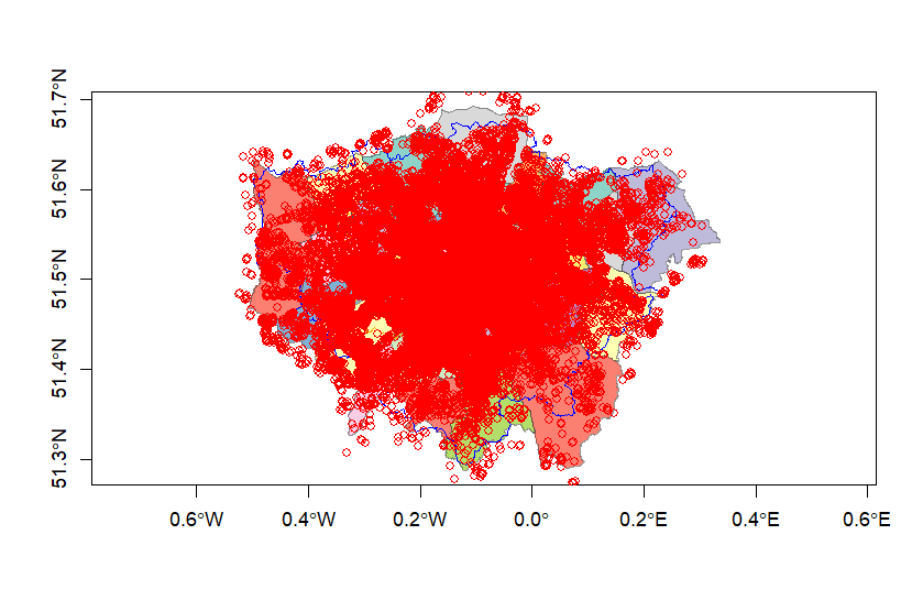
Plotting points using plot()

Add points using st_geometry()

plot(st_geometry(listings_geo), add=TRUE, col='red')

Plotting sf points.

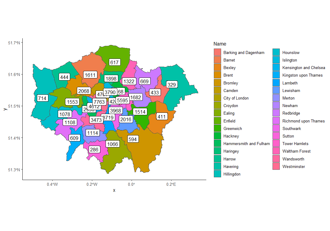
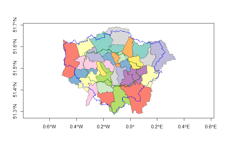
Plotting polygons using ggplot()

We can use ggplot() to plot layers of sf
Need to match up the coordinate reference system (CRS) for the two layers

Geospatial map created using ggplot.

num_listings <- listings %>% 
  group_by(neighbourhood) %>%
  summarize(`Number of listings` = n(),
            longitude = mean(longitude),
            latitude = mean(latitude),
            .groups = "drop") %>%

  st_as_sf(coords = c("longitude", "latitude"))

st_crs(num_listings) <- st_crs(london_poly)

ggplot_map <- ggplot(london_poly) + 
  geom_sf(aes(fill = Name)) +

  geom_sf_label(data=num_listings, 
              aes(label=`Number of listings`)) +
  theme_classic()

Let's practice!

Building Dashboards with shinydashboard