Shrinkage methods

Feature Engineering in R

Jorge Zazueta

Research Professor and Head of the Modeling Group at the School of Economics, UASLP

Two common regularization techniques

Lasso

Adds penalty term proportional to absolute value of model weights
Encourages some weights to become exactly zero
Effectively eliminates the corresponding features
Can be an automated feature selection method

Ridge

Adds penalty term proportional to square of model weights
Does not shrink some coefficients to zero like Lasso
But can effectively reduce overfitting

A first look at Lasso

Set up the model

recipe <- # Define recipe
recipe(Loan_Status ~ ., data = train) %>%
  step_normalize(all_numeric_predictors()) %>% 
  step_dummy(all_nominal_predictors()) %>%
  update_role(Loan_ID, new_role = "ID")
# set up model
model_lasso_manual <- logistic_reg() %>%
  set_engine("glmnet") %>%
  set_args(mixture = 1, penalty = .2)
# Bundle in workflow
workflow_lasso_manual <-
  workflow() %>%
  add_model(model_lasso_manual) %>%
  add_recipe(recipe)

Fit and inspect

fit_lasso_manual <- # Fit workflow
  workflow_lasso_manual %>% 
  fit(train)
#Inspect coefficients
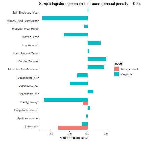
tidy(fit_lasso_manual)

# A tibble: 15 × 3
   term                    estimate penalty
   <chr>                      <dbl>   <dbl>
 1 (Intercept)               -0.816     0.2
 2 ApplicantIncome            0         0.2
 3 CoapplicantIncome          0         0.2
 4 LoanAmount                 0         0.2
 5 Loan_Amount_Term           0         0.2
 6 Credit_History            -0.220     0.2
 7 Gender_Female              0         0.2
 ...                          ...        ...

Simple logistic regression vs. Lasso

Column chart of simple logistic regression versus Lasso.

Hyperparameter tuning

Setting a model with tuning

model_lasso_tuned <- logistic_reg() %>%
  set_engine("glmnet") %>%
  set_args(mixture = 1, 
  penalty = tune()) 

workflow_lasso_tuned <-
  workflow() %>%
  add_model(model_lasso_tuned) %>%
  add_recipe(recipe)

penalty_grid <- grid_regular(
  penalty(range = c(-3, 1)),
  levels = 30)

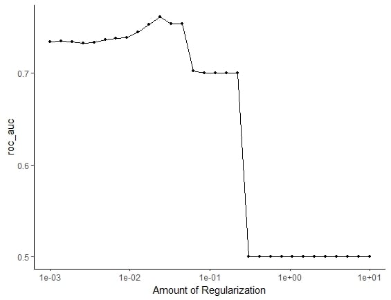
Looking at the tuning output

tune_output <- tune_grid( 
  workflow_lasso_tuned,
  resamples = vfold_cv(train, v = 5),
  metrics = metric_set(roc_auc),
  grid = penalty_grid)
autoplot(tune_output)

Chart of ROC_AUC versus amount of regulatization.

Exploring the results

Auto-chosen features

best_penalty <- 
select_by_one_std_err(tune_output, 
metric = 'roc_auc', desc(penalty)) 

# Fit Final Model
final_fit<- 
finalize_workflow(workflow_lasso_tuned, 
best_penalty) %>%
  fit(data = train)

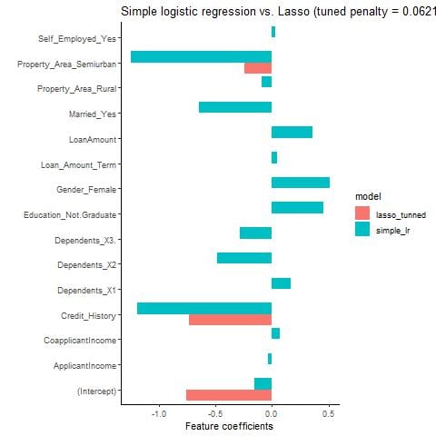
final_fit_se %>% tidy()

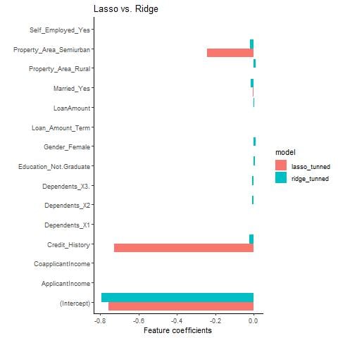
# A tibble: 15 × 3
   term                    estimate penalty
   <chr>                      <dbl>   <dbl>
 1 (Intercept)               -0.660  0.0452
 2 ApplicantIncome            0      0.0452
 3 CoapplicantIncome          0      0.0452
 4 LoanAmount                 0      0.0452
 5 Loan_Amount_Term           0      0.0452
 6 Credit_History            -0.948  0.0452
 7 Gender_Female              0      0.0452
 8 Married_Yes               -0.191  0.0452
 9 Dependents_X1              0      0.0452
10 Dependents_X2              0      0.0452
11 Dependents_X3.             0      0.0452
12 Education_Not.Graduate     0      0.0452
13 Self_Employed_Yes          0      0.0452
14 Property_Area_Rural        0      0.0452
15 Property_Area_Semiurban   -0.163  0.0452

Simple logistic regression vs. tuned Lasso

Ridge regularization

Ridge is the option when mixture = 0

model_ridge_tuned <- logistic_reg() %>%
  set_engine("glmnet") %>%
  set_args(mixture = 0, penalty = tune()) 

workflow_ridge_tuned <-
  workflow() %>%
  add_model(model_ridge_tuned) %>%
  add_recipe(recipe)

tune_output <- tune_grid( 
  workflow_ridge_tuned,
  resamples = vfold_cv(train, v = 5),
  metrics = metric_set(roc_auc),
  grid = penalty_grid)

tune_output <- tune_grid( 
  workflow_ridge_tuned,
  resamples = vfold_cv(train, v = 5),
  metrics = metric_set(roc_auc),
  grid = penalty_grid)  
 autoplot(tune_output)

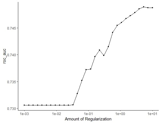
Ridge regularization

best_penalty <- 
select_by_one_std_err(tune_output,
metric = 'roc_auc', desc(penalty)) 
best_penalty

final_fit<- 
finalize_workflow(workflow_ridge_tuned, 
best_penalty) %>%
  fit(data = train)

tidy(final_fit)

# A tibble: 15 × 3
   term                      estimate penalty
   <chr>                        <dbl>   <dbl>
 1 (Intercept)             -0.799          10
 2 ApplicantIncome          0.00232        10
 3 CoapplicantIncome        0.0000537      10
 4 LoanAmount               0.00291        10
 5 Loan_Amount_Term         0.00161        10
 6 Credit_History          -0.0245         10
 7 Gender_Female            0.00850        10
 8 Married_Yes             -0.0140         10
 9 Dependents_X1            0.00497        10
10 Dependents_X2           -0.0100         10
11 Dependents_X3.           0.00259        10
12 Education_Not.Graduate   0.00308        10
13 Self_Employed_Yes        0.00892        10
14 Property_Area_Rural      0.0109         10
15 Property_Area_Semiurban -0.0139         10

Ridge vs. Lasso

Let's practice!

Feature Engineering in R