Reducing dimensionality

Feature Engineering in R

Jorge Zazueta

Research Professor and Head of the Modeling Group at the School of Economics, UASLP

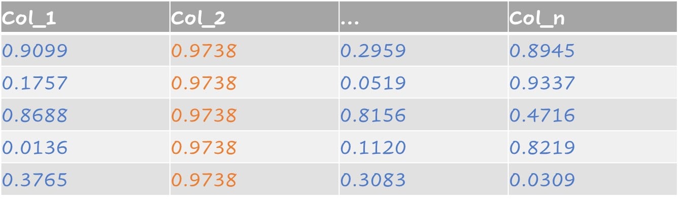
Zero variance features

Some datasets include columns with constant values or zero variance. We can filter out those features by adding step_zv() to our recipe().

Table illustrating a feature with zero variance.

Near-zero variance features

Near-zero variance features include predictors with a single value and predictors with both of the following characteristics:

Very few unique values relative to the number of samples
The ratio of the frequency of the most common value to the frequency of the second most common value is large

Example of near-zero variance:

For 100 observations there are two different values but one occurs only once.

step_nzv() identifies and removes predictors with these characteristics.

Principal Component Analysis (PCA)

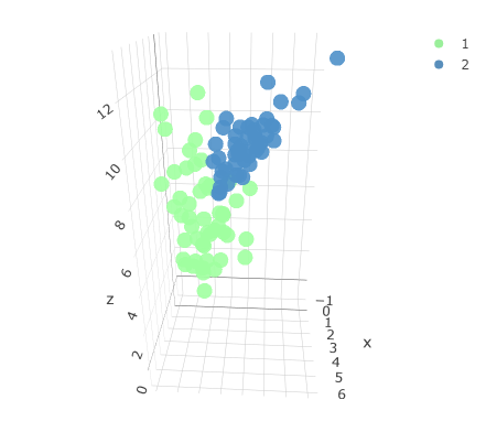
Original three-dimensional dataset with two associated classes.

A three-dimensional graph with two data classes.

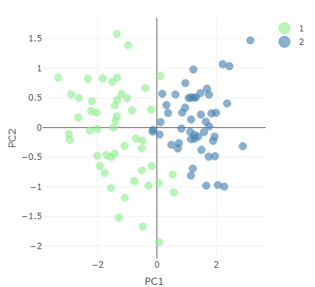
Reduced dataset representing data using first two principal components.

A two-dimensional graph showing two data classes as a scatterplot of the first two principal components.

Let's prep a recipe

Creating a recipe to perform PCA and retrieving its output via prep().

pc_recipe <- 
recipe(~., data = loans_num) %>%
  step_nzv(all_numeric()) %>%
  step_normalize(all_numeric()) %>%
  step_pca(all_numeric())

pca_output <- prep(pc_recipe)

We can look at the information available by calling names() on pca_output.

names(pca_output)

 [1] "var_info"       "term_info"     
 [3] "steps"          "template"      
 [5] "levels"         "retained"      
 [7] "requirements"   "tr_info"       
 [9] "orig_lvls"      "last_term_info"

Unearthing variance explained

Extract standard deviation from the pca_output object and compute variance explained.

stdv <- pca_output$steps[[3]]$res$sdev

var_explained <- stdv^2/sum(stdv^2)

PCA = tibble(PC = 1:length(stdv),
          var_explained = var_explained, 
          cumulative = cumsum(var_explained))

A table showing variance explained by principal component.

# A tibble: 5 × 3
     PC var_explained cumulative
  <int>         <dbl>      <dbl>
1     1        0.315       0.315
2     2        0.214       0.529
3     3        0.202       0.730
4     4        0.198       0.928
5     5        0.0722      1

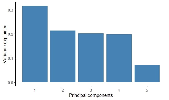
Visualizing variance explained

We can graph the output as a column chart using ggplot2.

PCA %>% 
ggplot(aes(x = PC, 
           y = var_explained)) +
  geom_col(fill = "steelblue") +
  xlab("Principal components") +
  ylab("Variance explained")

Variance explained by principal component.

Column chart showing variance explained by principal component.

Let's practice!

Feature Engineering in R