Mann-Whitney U test
A/B Testing in R

Lauryn Burleigh
Data Scientist
Mann-Whitney U
Assumptions
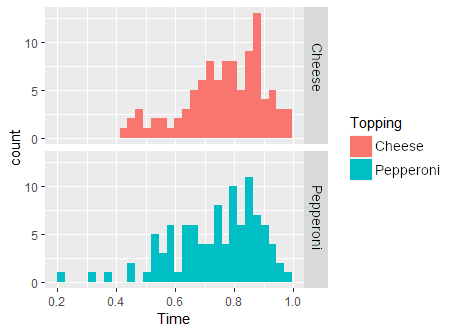
library(ggplot2)
ggplot(pizza, aes(x = Time,
                  fill = Topping)) +
       geom_histogram() +
       facet_grid(Topping~.)
A/B Testing in R
Lauryn Burleigh
Data Scientist
library(ggplot2)
ggplot(pizza, aes(x = Time,
fill = Topping)) +
geom_histogram() +
facet_grid(Topping~.)

