Measuring the benefits

Parallel Programming in R

Nabeel Imam

Data Scientist

Toy example

numbers <- 1:1000000


# Sequential
sqroots <- lapply(numbers, sqrt)


# Parallel
cl <- makeCluster(4)
sqroots <- parLapply(cl, numbers, sqrt)
stopCluster(my_cluster)

Which will perform better?

Benchmarking performance

Run code several times to estimate average execution time

library(microbenchmark)


microbenchmark(
  "Sequential" = lapply(numbers, sqrt),

  "Parallel" = {
    cl <- makeCluster(4)
    parLapply(cl, numbers, sqrt)
    stopCluster(my_cluster)
  },

  times = 10
)

Unit: milliseconds
      expr     min    mean     max neval
Sequential  633.96  838.09  993.59    10
  Parallel 1136.95 1247.29 1557.58    10

Simple numerical operations rarely benefit from parallelization
Profiling gives line-by-line report, benchmarking gives overall execution times

The elephant in the room

sqroots <- sqrt(numbers)

An elephant sits on the couch in a living room and people acknowledge its presence.

Vectorization

sqroots <- sqrt(numbers)

Base R functions, like sqrt(), are vectorized.
Map a single function to many inputs
Very fast but only applicable to simple operations

microbenchmark(
  "Vectorized" = sqrt(numbers),
  "Sequential" = lapply(numbers, sqrt),
  "Parallel" = {
    cl <- makeCluster(4)
    parLapply(cl, numbers, sqrt)
    stopCluster(my_cluster)
  },
  times = 10)

Unit: milliseconds
      expr       min      mean      max neval
Vectorized    2.3904    9.2071   66.303    10
Sequential  352.1166  771.7491 1004.753    10
  Parallel 1191.3176 1377.6926 1700.316    10

The bootstrap

Sampling from the current data with replacement

print(ls_df)

$`2001`
   Country             Life_expectancy  Year
 1 Afghanistan                    56.3  2001
 2 Albania                        74.3  2001
 3 Algeria                        71.1  2001
...
$`2002`
   Country             Life_expectancy  Year
 1 Afghanistan                    56.8  2002
 2 Albania                        74.6  2002
 3 Algeria                        71.6  2002
...

Classic version

df <- ls_df$`2001`


estimates <- rep(0, 10000)


for (i in 1:10000) {

  b <- sample(df$Life_expectancy,
              replace = T)


  estimates[i] <- mean(b)
  }

A histogram of bootstrapped estimates of the global average life expectancy in 2001, showing the classic bell curve.

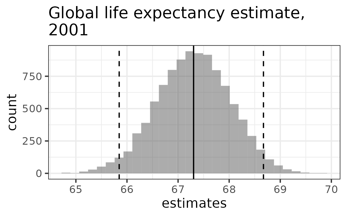
Confidence interval using quantiles: quantile(estimates, c(0.025, 0.975))

The good news

Bootstraps can be parallelized

estimates <- rep(0, 10000)

for (i in 1:10000) {

  b <- sample(df$Life_expectancy,
              replace = T)

  estimates[i] <- mean(b)
  }

boot_dist <- function (df) {

  estimates <- rep(0, 10000)

  for (i in 1:10000) {
    b <- sample(df$Life_expectancy, replace = T)
    estimates[i] <- mean(b)
  }

  return(estimates)
}


cl <- makeCluster(4)
ls_dists <- parLapply(cl, ls_df, boot_dist)
stopCluster(cl)

The benefits

microbenchmark(
  "lapply" = lapply(ls_df, boot_dist),
  "parLapply" = {
    cl <- makeCluster(4)
    parLapply(cl, ls_df, boot_dist)
    stopCluster(cl)
  },
  times = 10
)

Unit: seconds
     expr    min   mean    max neval
   lapply 3.6938 4.2184 4.5267    10
parLapply 1.9006 2.5166 2.7292    10

How to get there:

Profile existing code, identify slowest part
Parallelize/optimize this step
Benchmark and compare

Let's practice!

Parallel Programming in R