Working with a forecast object

Designing Forecasting Pipelines for Production

Rami Krispin

Senior Manager, Data Science and Engineering

Work with a forecast object

Data preparation
Train and test multiple forecasting models
Evaluate the models' performance
The statsforecast package
- mlforecast in the exercises

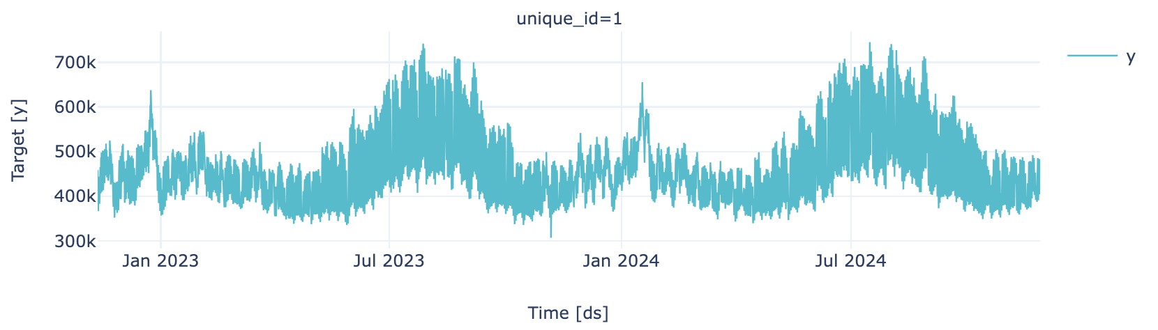
Training Partition

Time Series

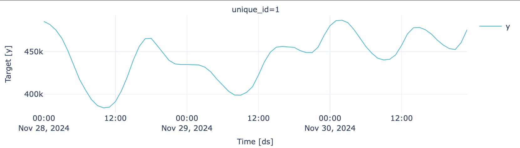
Testing Partition

Required libraries

import pandas as pd 
import datetime

Required libraries

from statsforecast import StatsForecast

from statsforecast.models import (
    DynamicOptimizedTheta,
    SeasonalNaive,
    AutoARIMA,
    HoltWinters,
    MSTL
)

from utilsforecast.plotting import plot_series

The statsforecast data format

Data input format:

unique_id - the series ID
ds - the series timestamp
y - the series values

Data preparation - data load

ts = pd.read_csv("data/data.csv")
ts["ds"] = pd.to_datetime(ts["ds"])
ts = ts.sort_values("ds")
ts = ts[["unique_id", "ds", "y"]]

os.environ['NIXTLA_ID_AS_COL'] = '1'

 unique_id        ds             y
0    1    2022-11-11 23:00:00    456403
1    1    2022-11-12 00:00:00    458842
2    1    2022-11-12 01:00:00    455111
3    1    2022-11-12 02:00:00    448035
4    1    2022-11-12 03:00:00    438165

Data preparation - train/test split

Split the time series into training and testing partitions
- using datetime.timedelta
- leave last 72 hours as test data

test_length = 72

train_end = end  - datetime.timedelta(hours = test_length)

train = ts[ts["ds"] <= train_end]
test = ts[ts["ds"] > train_end]

Data preparation

plot_series(train, engine = "plotly")

Time Series

plot_series(test, engine = "plotly")

Testing Partition

Forecasting with StatsModels

# Instantiate models with hourly seasonality
auto_arima = AutoARIMA()
s_naive = SeasonalNaive(season_length=24)
theta =  DynamicOptimizedTheta(season_length=24)


# Instantiate models with hourly and weekly seasonality
mstl1 = MSTL(season_length=[24, 24 * 7], 
            trend_forecaster=AutoARIMA(),
            alias="MSTL_ARIMA_trend")

mstl2 = MSTL(season_length=[24, 24 * 7], 
            trend_forecaster=HoltWinters(),
            alias="MSTL_Holt_trend")

Forecasting with StatsModels

# Combine models into a list
stats_models = [auto_arima, s_naive, theta, mstl1, mstl2]


# Instantiate the model object
sf = StatsForecast( 
    models=stats_models,
    freq="h", 
    fallback_model = AutoARIMA(),
    n_jobs= -1)

Forecasting with StatsModels

# Combine models into a list
stats_models = [auto_arima, s_naive, theta, mstl1, mstl2]


# Instantiate the model object
sf = StatsForecast( 
    models=stats_models,
    freq="h", 
    fallback_model = AutoARIMA(),
    n_jobs= -1)


# Create the forecast
forecast_stats = sf.forecast(df=train, h=72, level=[95])

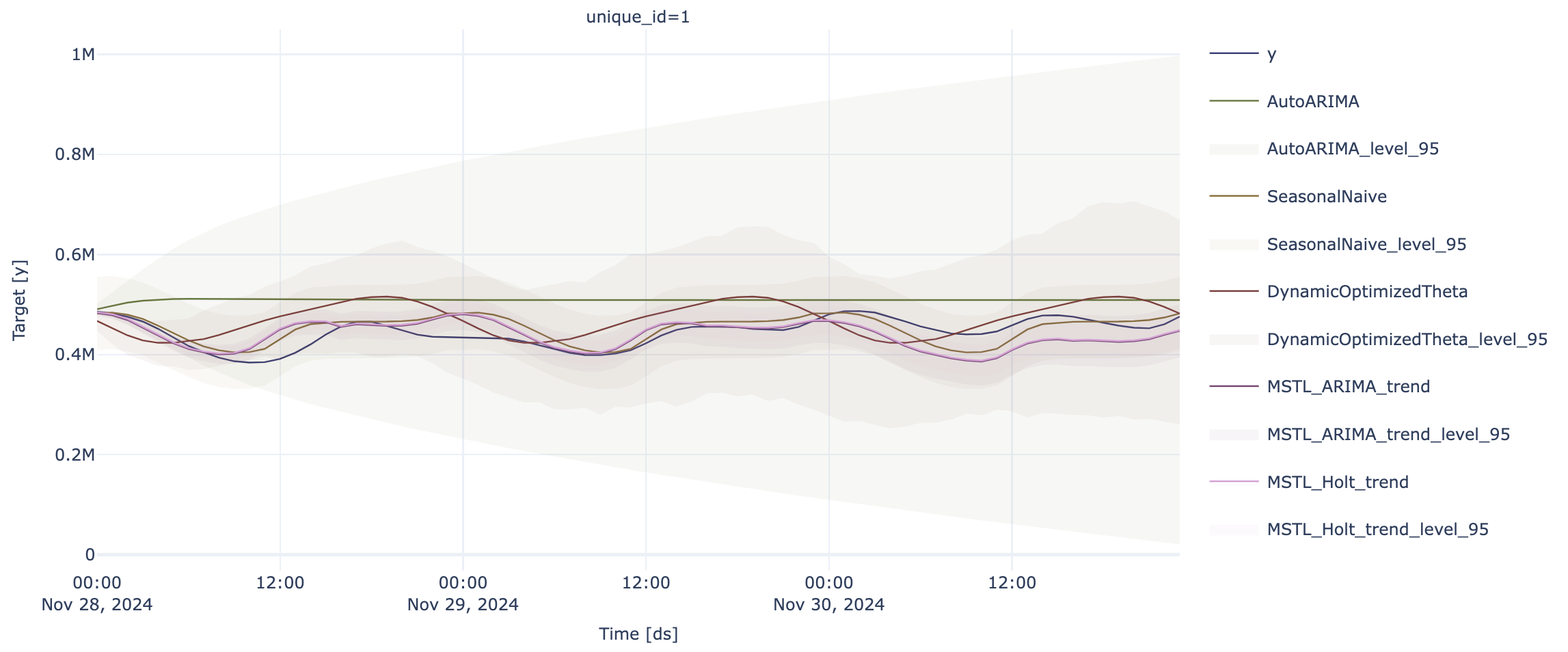
Forecast Forecasting with StatsModels StatsModels

p = sf.plot(test, forecast_stats, engine = "plotly", level=[95])
p.update_layout(height=400)

Forecast Plot

Model evaluation

def mape(y, yhat):
    mape = mean(abs(y - yhat)/ y) 
    return mape

def rmse(y, yhat):
    rmse = (mean((y - yhat) ** 2 )) ** 0.5
    return rmse

def coverage(y, lower, upper):
    coverage = sum((y <= upper) & (y >= lower)) / len(y)
    return coverage

Model evaluation

fc = forecast_stats.merge(test, how="left", on="ds")
fc_performance = None

for i in [str(m) for m in stats_models]:
    m = mape(y = fc["y"], yhat = fc[i])
    r = rmse(y = fc["y"], yhat = fc[i])
    c = coverage(y = fc["y"], lower = fc[i + "-lo-95"], upper = fc[i + "-hi-95"])

    perf = {"model": i,
            "mape": m,
            "rmse": r,
            "coverage": c}
    if fc_performance is None:
        fc_performance = pd.DataFrame([perf])
    else:
        fc_performance = pd.concat([fc_performance, pd.DataFrame([perf])])
fc_performance.reset_index(drop=True, inplace=True)

Model evaluation

print(fc_performance.sort_values("rmse"))

     model                    mape        rmse            coverage
1    SeasonalNaive            0.041340    22410.483959    1.000000
4    MSTL_Holt_trend          0.053939    30201.299395    0.513889
3    MSTL_ARIMA_trend         0.053771    30428.240235    0.666667
2    DynamicOptimizedTheta    0.090566    45189.869437    0.916667
0    AutoARIMA                0.149790    70483.617198    1.000000

Model evaluation

print(fc_performance.sort_values("rmse"))

     model                    mape        rmse            coverage
1    SeasonalNaive            0.041340    22410.483959    1.000000
4    MSTL_Holt_trend          0.053939    30201.299395    0.513889
3    MSTL_ARIMA_trend         0.053771    30428.240235    0.666667
2    DynamicOptimizedTheta    0.090566    45189.869437    0.916667
0    AutoARIMA                0.149790    70483.617198    1.000000

Can we improve the results?

Different settings for better accuracy
Experiments come in handy

Let's practice!

Designing Forecasting Pipelines for Production