Visualizar datos resumidos
Introducción a Tidyverse

David Robinson
Chief Data Scientist, DataCamp
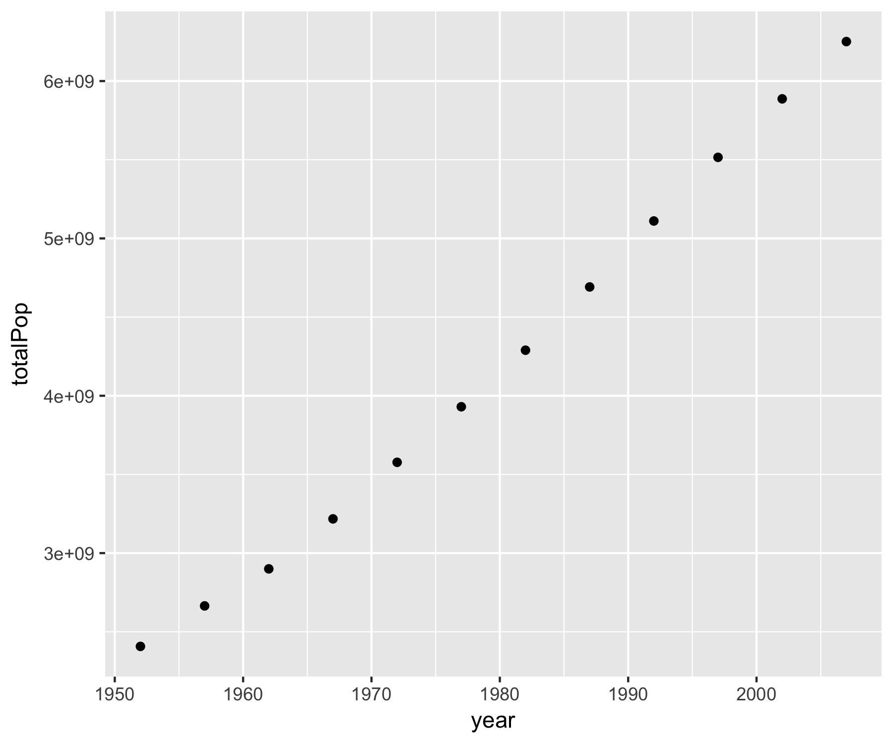
Visualización de la población a lo largo del tiempo
ggplot(by_year, aes(x = year, y = totalPop)) +
  geom_point()
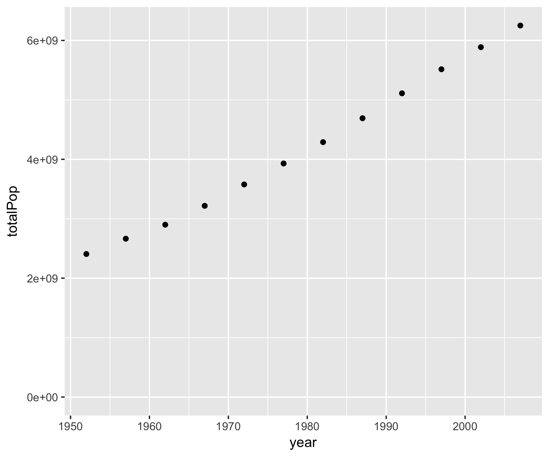
Eje y inicial en cero
ggplot(by_year, aes(x = year, y = totalPop)) +
  geom_point() +
  expand_limits(y = 0)
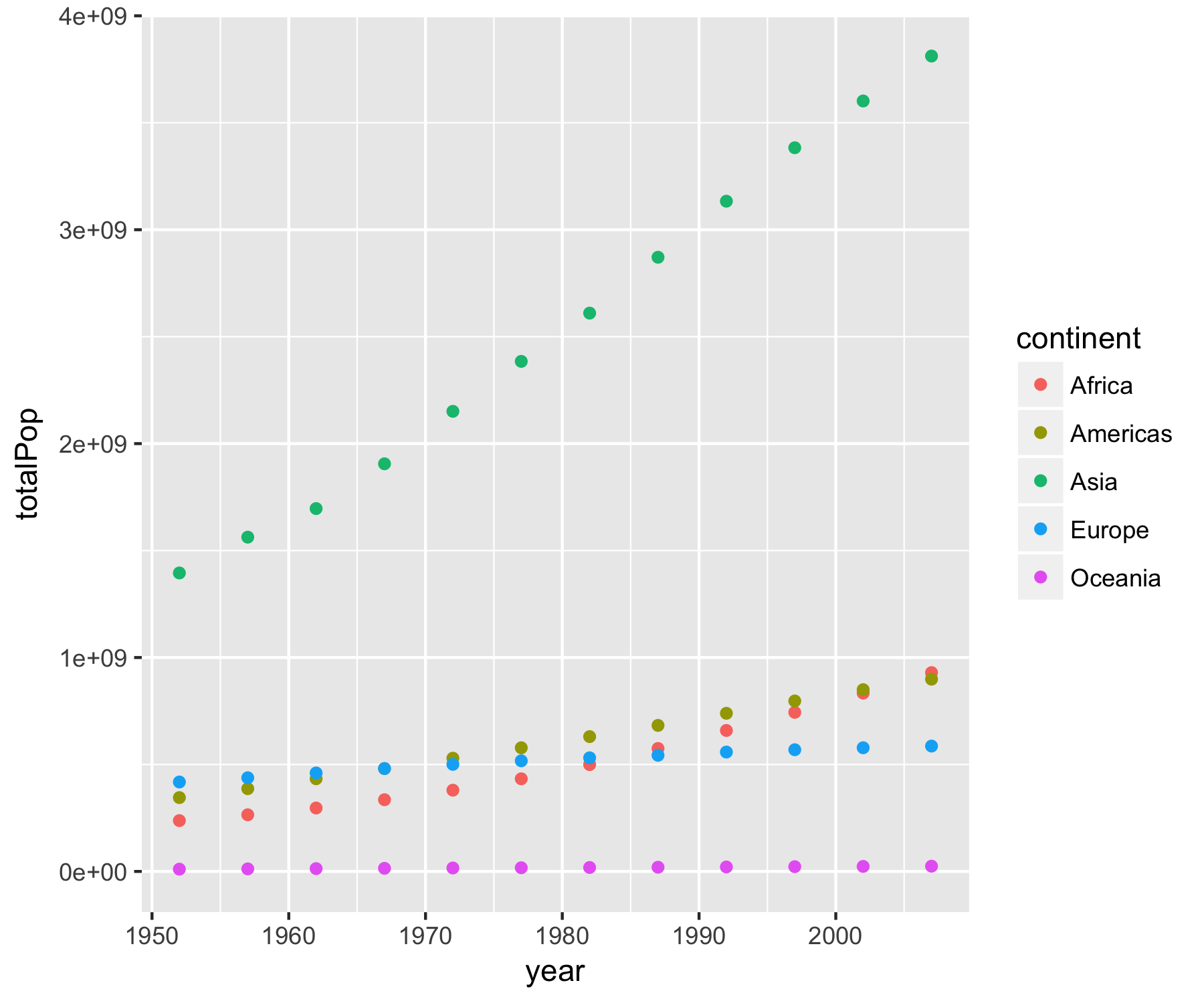
Visualización de la población por año y continente
ggplot(by_year_continent, aes(x = year, y = totalPop, color = continent)) +
  geom_point() +
  expand_limits(y = 0)