Introduction to the Tidyverse
David Robinson
Chief Data Scientist, DataCamp
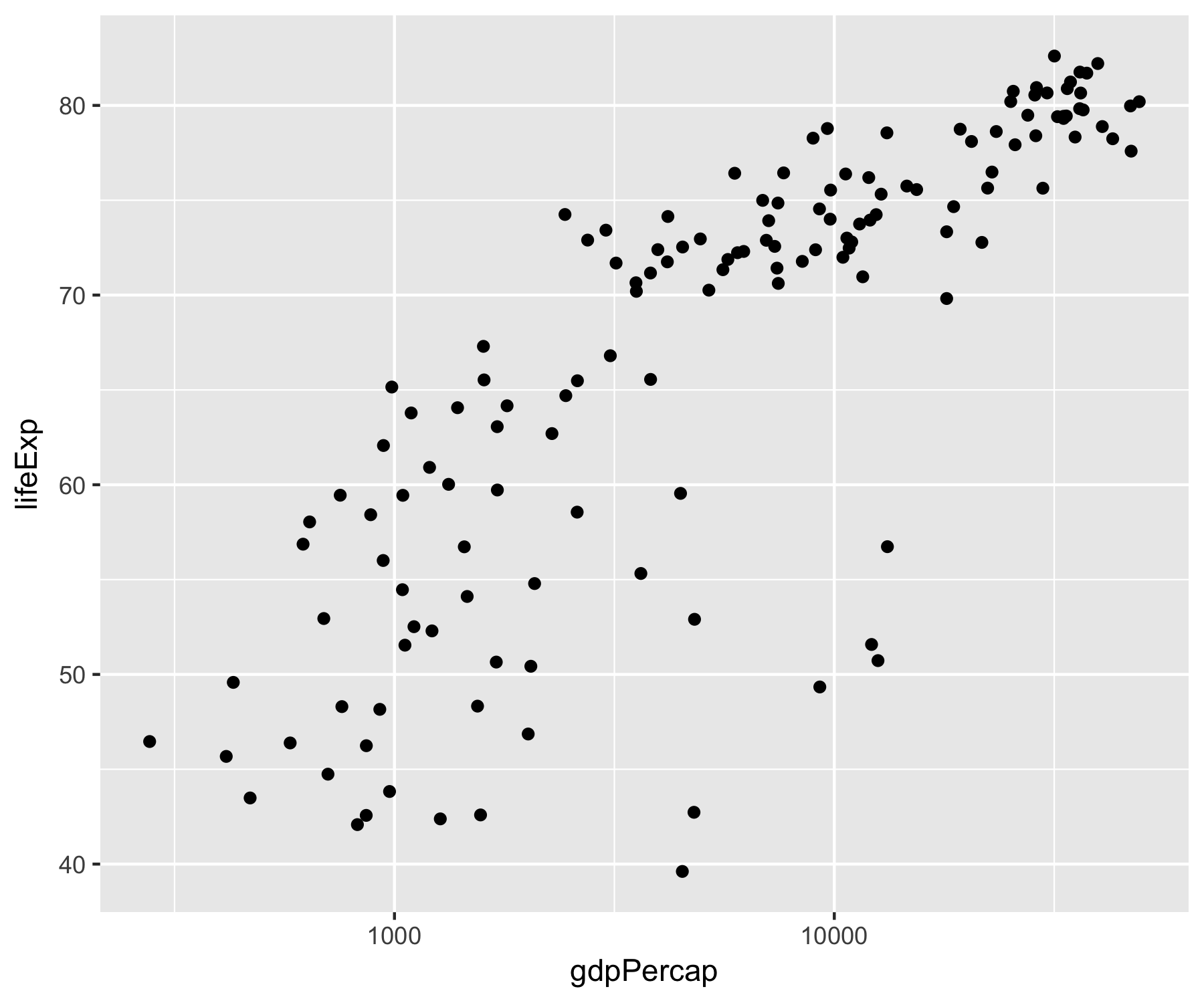
gapminder_2007
# A tibble: 142 x 6
country continent year lifeExp pop gdpPercap
<fct> <fct> <int> <dbl> <dbl> <dbl>
1 Afghanistan Asia 2007 43.828 31889923 974.5803
2 Albania Europe 2007 76.423 3600523 5937.0295
3 Algeria Africa 2007 72.301 33333216 6223.3675
4 Angola Africa 2007 42.731 12420476 4797.2313
5 Argentina Americas 2007 75.320 40301927 12779.3796
6 Australia Oceania 2007 81.235 20434176 34435.3674
7 Austria Europe 2007 79.829 8199783 36126.4927
8 Bahrain Asia 2007 75.635 708573 29796.0483
9 Bangladesh Asia 2007 64.062 150448339 1391.2538
10 Belgium Europe 2007 79.441 10392226 33692.6051
# ... with 132 more rows
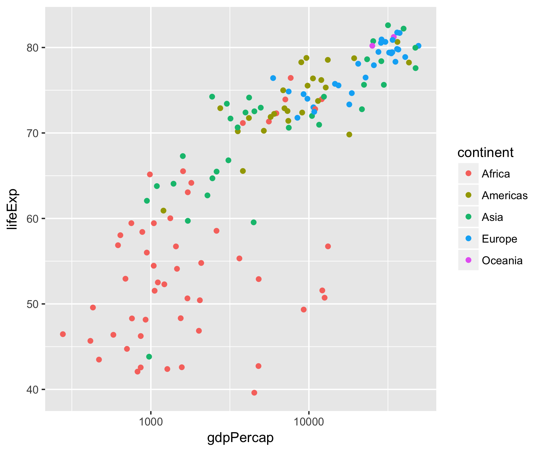
ggplot(gapminder_2007, aes(x = gdpPercap, y = lifeExp, color = continent)) +
geom_point() +
scale_x_log10()
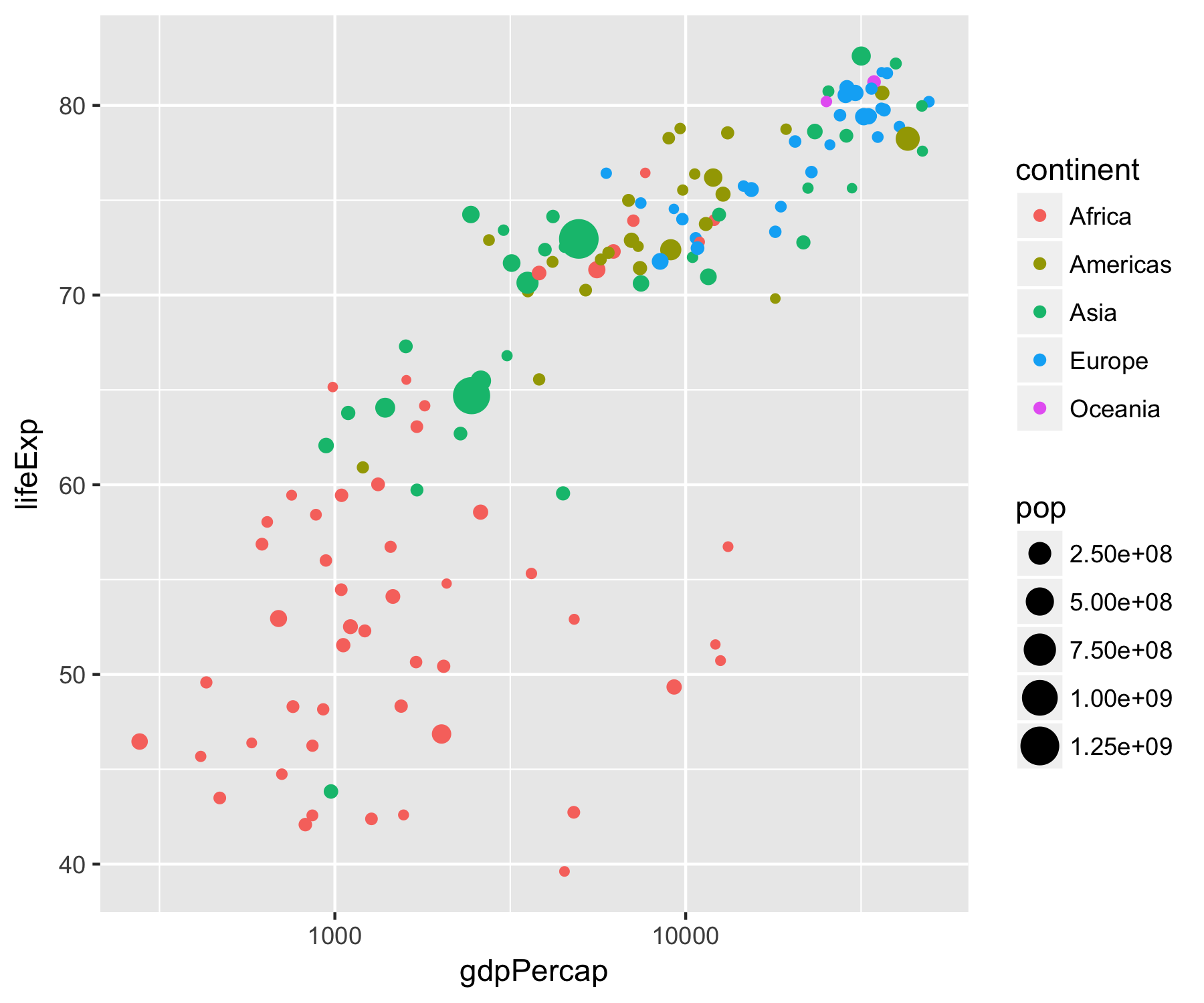
ggplot(gapminder_2007, aes(x = gdpPercap, y = lifeExp, color = continent,
size = pop)) +
geom_point() +
scale_x_log10()
Aesthetic | Variable |
---|---|
x | gdpPerCap |
y | lifeExp |
color | continent |
size | pop |
Introduction to the Tidyverse