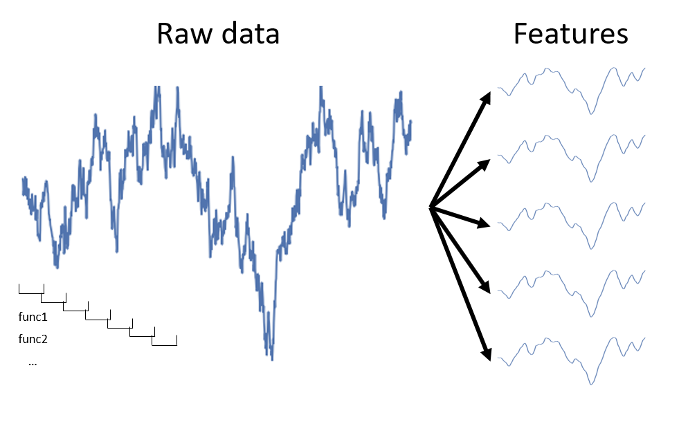
Creating features over time

Machine Learning for Time Series Data in Python

Chris Holdgraf

Fellow, Berkeley Institute for Data Science

Extracting features with windows

Using .aggregate for feature extraction

# Visualize the raw data
print(prices.head(3))

symbol            AIG        ABT
date                            
2010-01-04  29.889999  54.459951
2010-01-05  29.330000  54.019953
2010-01-06  29.139999  54.319953

# Calculate a rolling window, then extract two features
feats = prices.rolling(20).aggregate([np.std, np.max]).dropna()
print(feats.head(3))

                 AIG                  ABT           
                 std       amax       std       amax
date                                                
2010-02-01  2.051966  29.889999  0.868830  56.239949
2010-02-02  2.101032  29.629999  0.869197  56.239949
2010-02-03  2.157249  29.629999  0.852509  56.239949

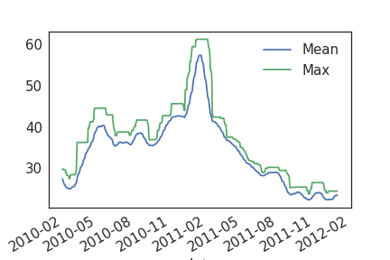
Check the properties of your features!

Using partial() in Python

# If we just take the mean, it returns a single value
a = np.array([[0, 1, 2], [0, 1, 2], [0, 1, 2]])
print(np.mean(a))

1.0

# We can use the partial function to initialize np.mean 
# with an axis parameter
from functools import partial
mean_over_first_axis = partial(np.mean, axis=0)

print(mean_over_first_axis(a))

[0. 1. 2.]

Percentiles summarize your data

Percentiles are a useful way to get more fine-grained summaries of your data (as opposed to using np.mean)
For a given dataset, the Nth percentile is the value where N% of the data is below that datapoint, and 100-N% of the data is above that datapoint.

print(np.percentile(np.linspace(0, 200), q=20))

40.0

Combining np.percentile() with partial functions to calculate a range of percentiles

data = np.linspace(0, 100)

# Create a list of functions using a list comprehension
percentile_funcs = [partial(np.percentile, q=ii) for ii in [20, 40, 60]]

# Calculate the output of each function in the same way
percentiles = [i_func(data) for i_func in percentile_funcs]
print(percentiles)

[20.0, 40.00000000000001, 60.0]

# Calculate multiple percentiles of a rolling window
data.rolling(20).aggregate(percentiles)

Calculating "date-based" features

Thus far we've focused on calculating "statistical" features - these are features that correspond statistical properties of the data, like "mean", "standard deviation", etc
However, don't forget that timeseries data often has more "human" features associated with it, like days of the week, holidays, etc.
These features are often useful when dealing with timeseries data that spans multiple years (such as stock value over time)

datetime features using Pandas

# Ensure our index is datetime
prices.index = pd.to_datetime(prices.index)

# Extract datetime features
day_of_week_num = prices.index.weekday
print(day_of_week_num[:10])

Index([0 1 2 3 4 0 1 2 3 4], dtype='object')

day_of_week = prices.index.weekday_name
print(day_of_week[:10])

Index(['Monday' 'Tuesday' 'Wednesday' 'Thursday' 'Friday' 'Monday' 'Tuesday'
 'Wednesday' 'Thursday' 'Friday'], dtype='object')

Let's practice!

Machine Learning for Time Series Data in Python