Medidas de dispersión
Introducción a la estadística

George Boorman
Curriculum Manager, DataCamp
¿Qué es la dispersión?
¿Por qué es importante la dispersión?

1 Crédito de la imagen: https://unsplash.com/@uyk
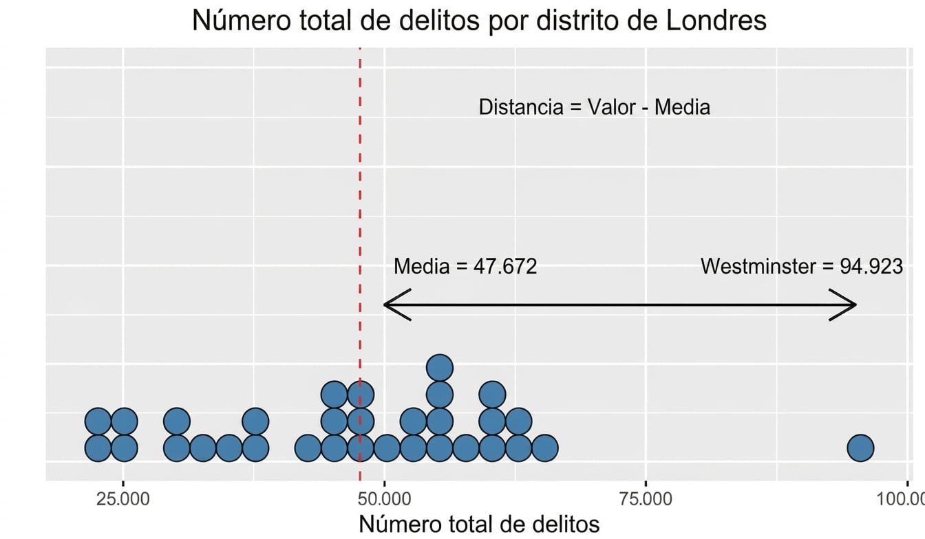
Varianza
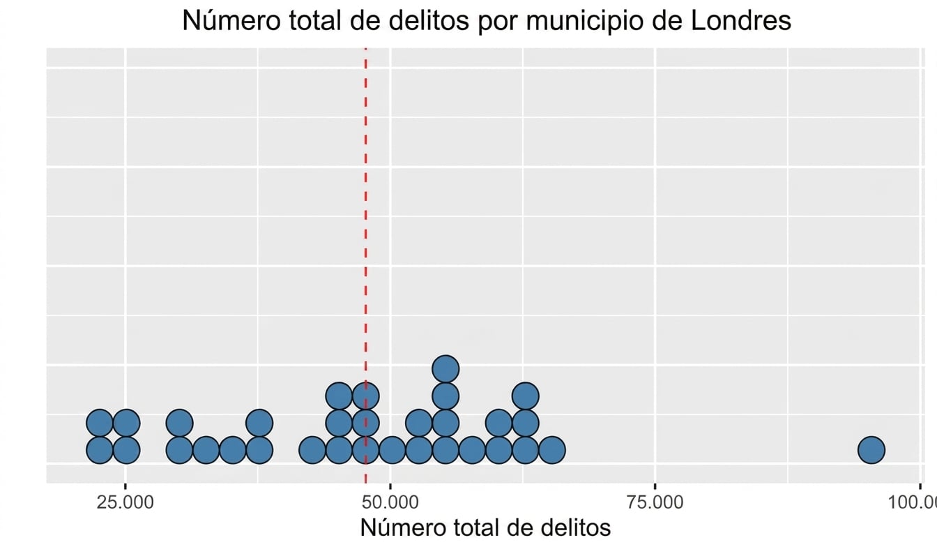
Varianza
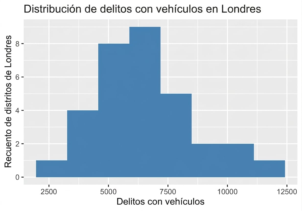
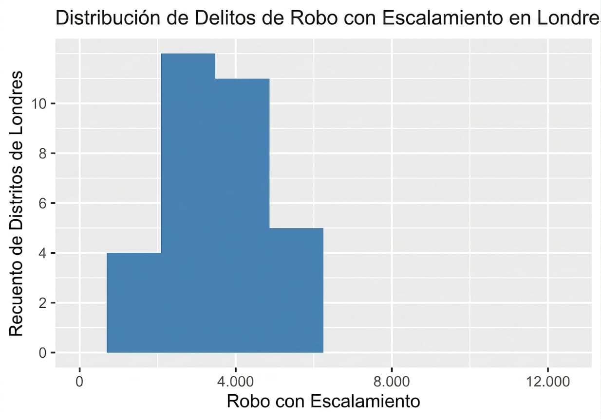
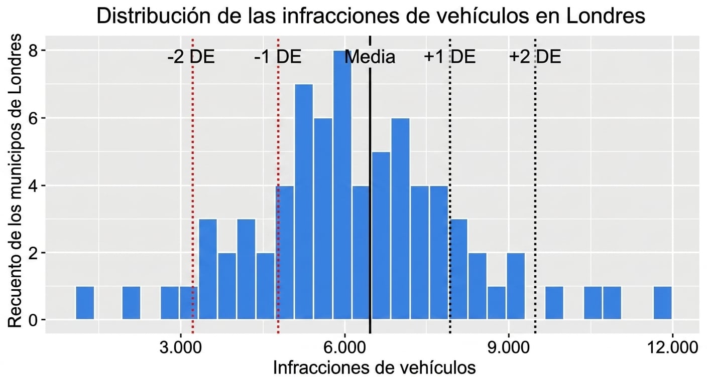
Desviación típica en un histograma
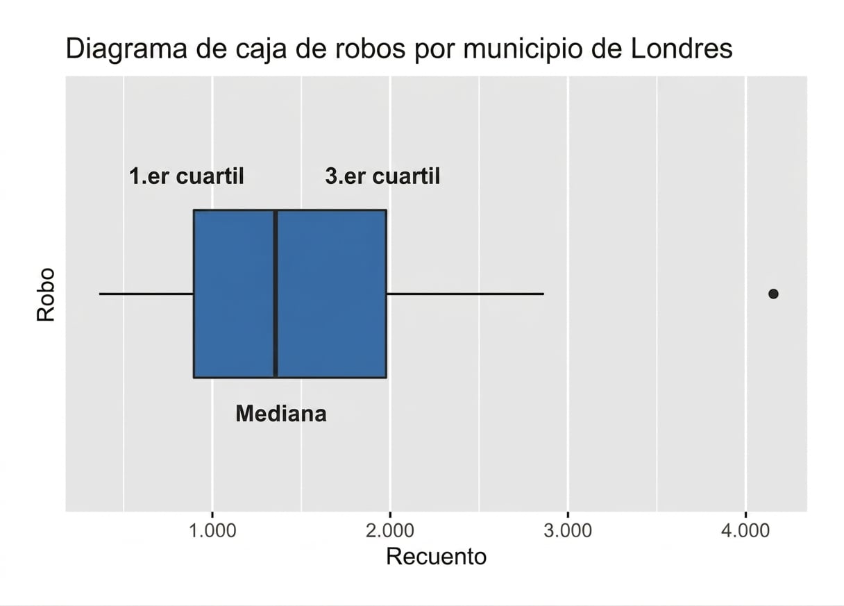
Diagramas de caja
Intervalo intercuartílico (IQR)
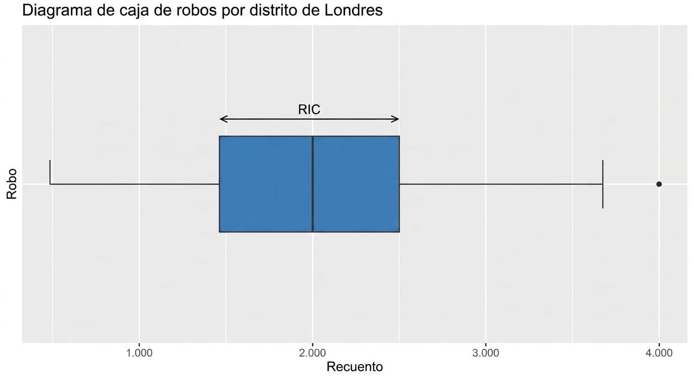
- El IQR se ve menos afectado por los valores extremos

