Advertencias sobre la correlación
Introducción a la estadística en R

Maggie Matsui
Content Developer, DataCamp
Relaciones no lineales
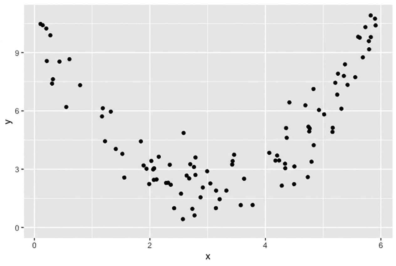
$$r = 0.18$$
Relaciones no lineales
Lo que vemos:
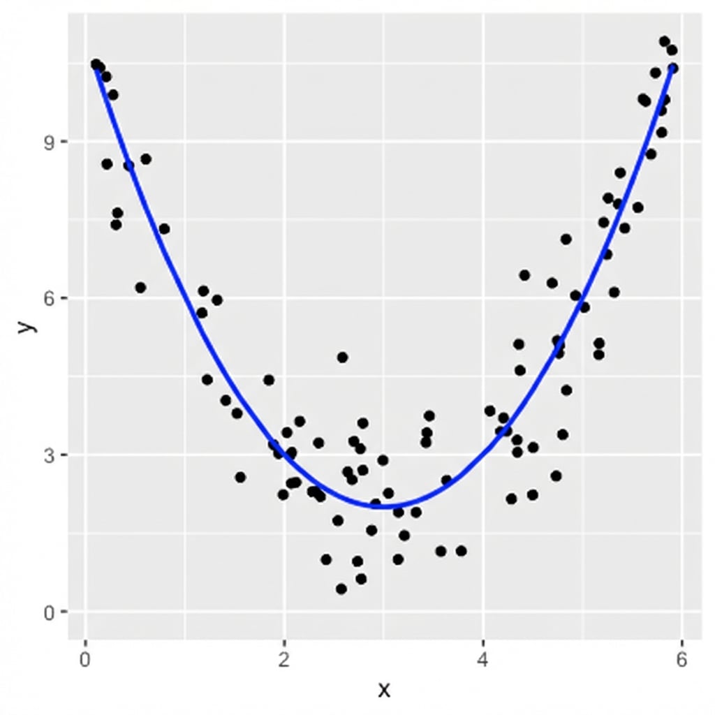
Lo que ve el coeficiente de correlación:
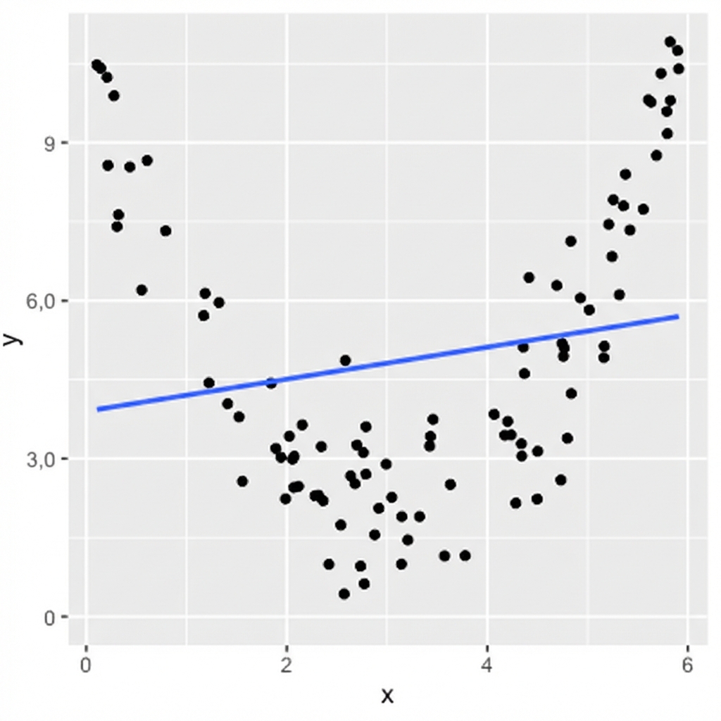
La correlación solo tiene en cuenta las relaciones lineales
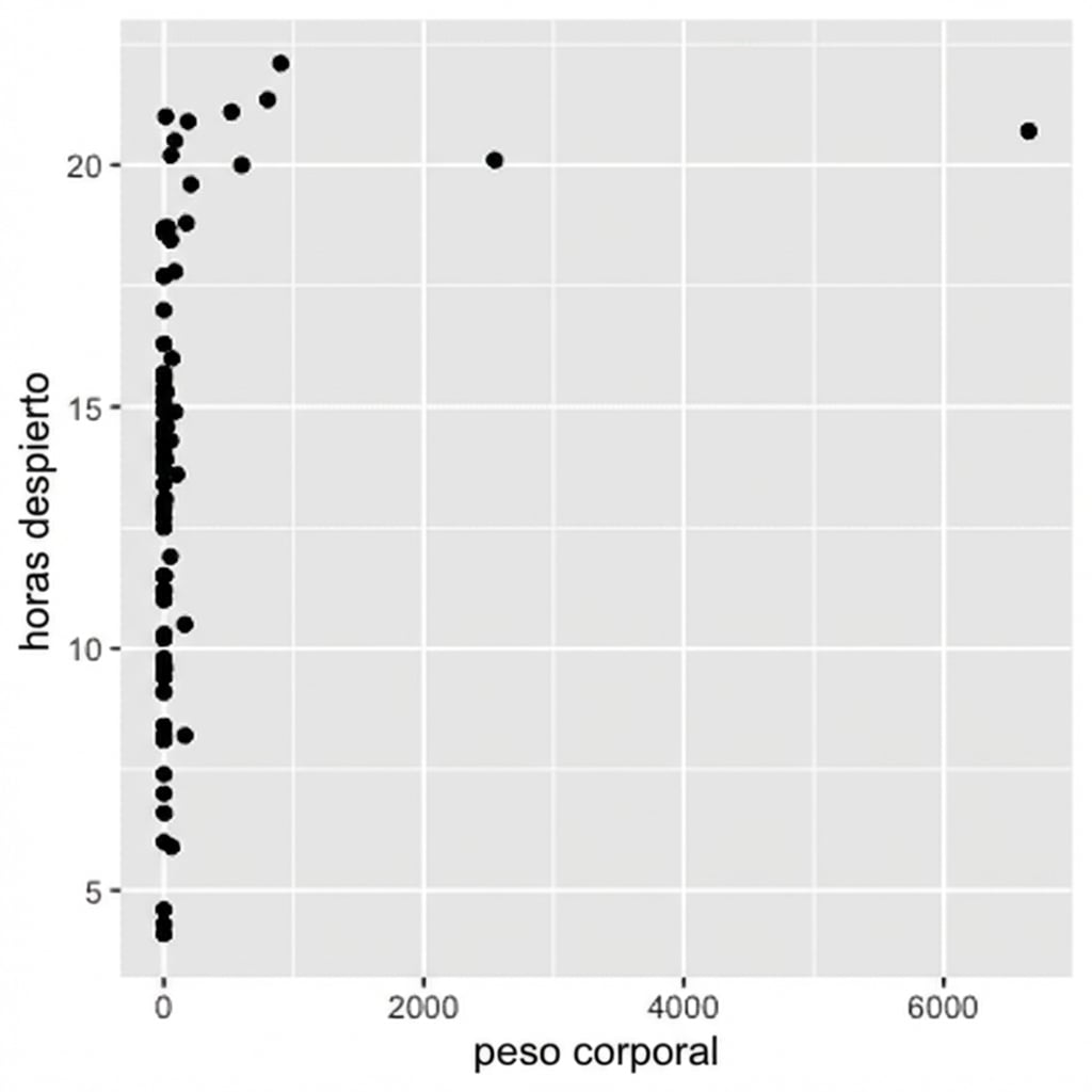
Visualiza siempre tus datos
Peso corporal frente a tiempo de vigilia
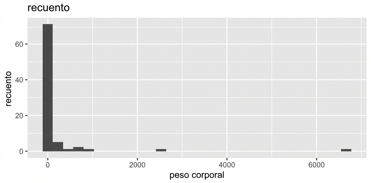
Distribución del peso corporal
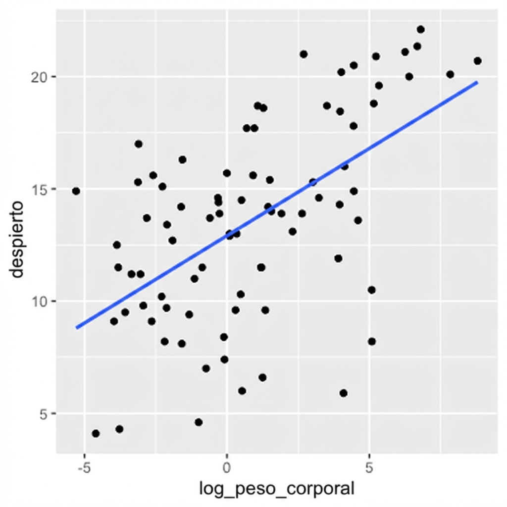
Transformación logarítmica
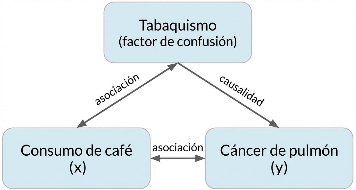
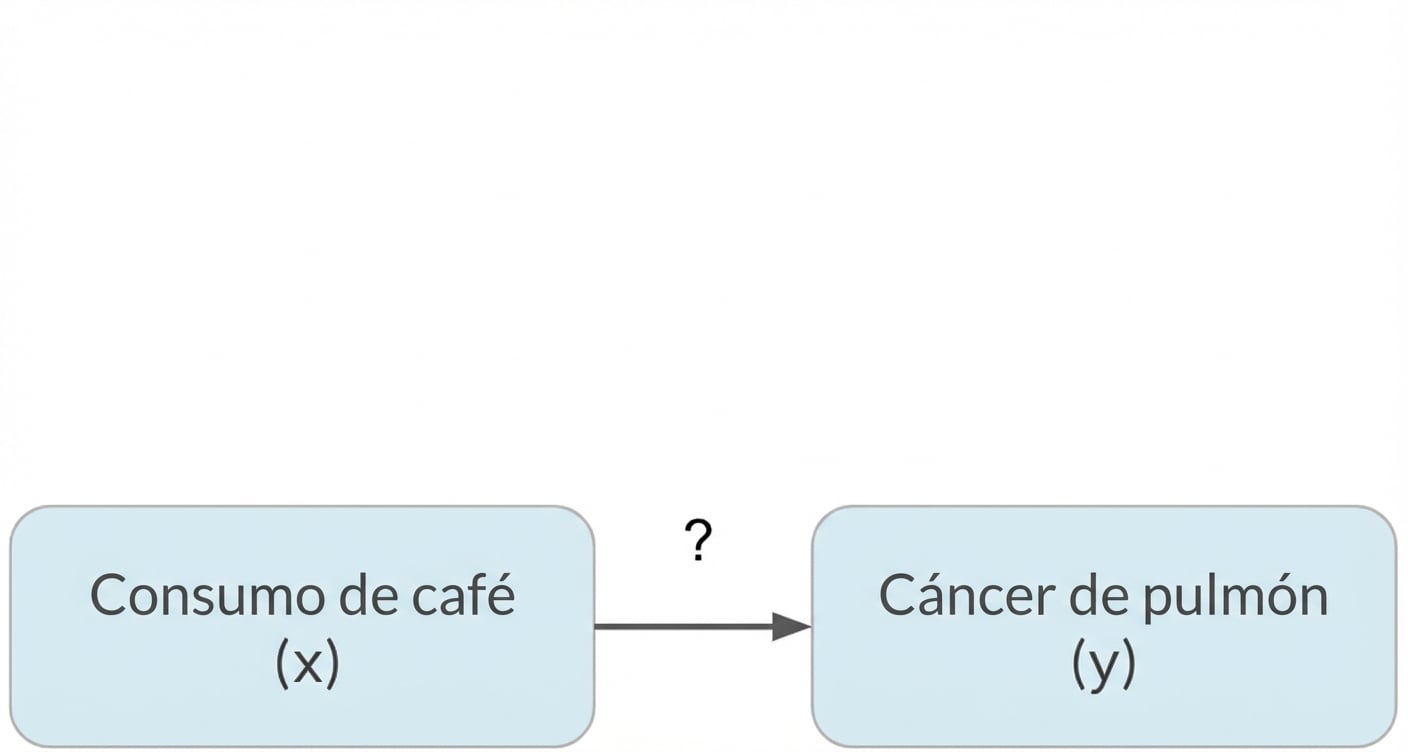
La correlación no implica causalidad
x está correlacionado con y no significa x que cause y

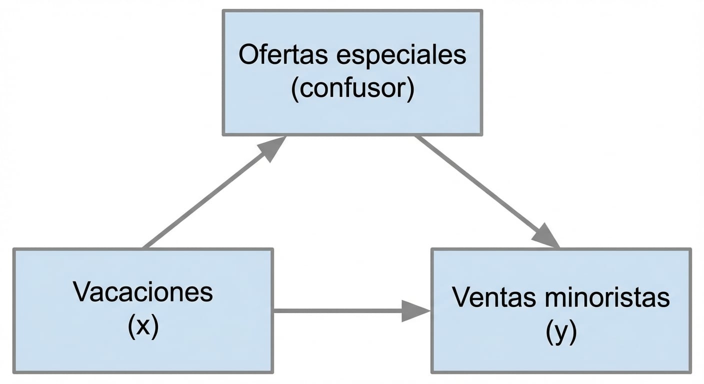
Confusión
Confusión

Confusión
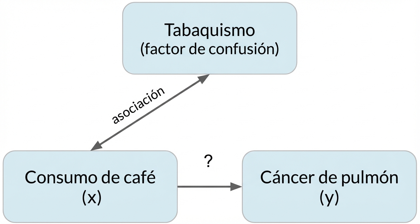
Confusión
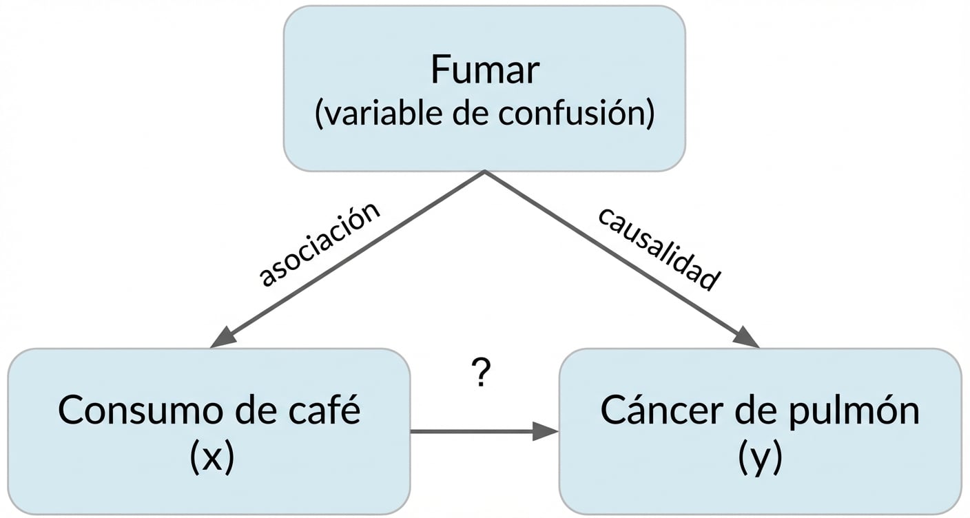
Confusión