El teorema del límite central
Introducción a la estadística en R

Maggie Matsui
Content Developer, DataCamp
Tirar los dados 5 veces

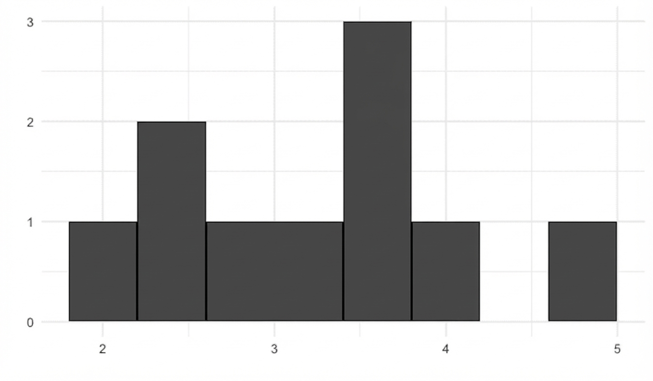
Distribuciones muestrales
Distribución muestral de la media muestral
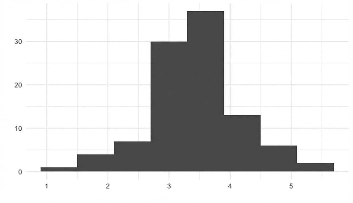
100 medias muestrales
replicate(100, sample(die, 5, replace = TRUE) %>% mean())
2.8 3.2 1.8 4.6 4.0 2.8 4.4 2.4 3.4 2.8 4.2 3.4 ... 2.2 3.8 3.6 3.8 4.4 4.8 2.4
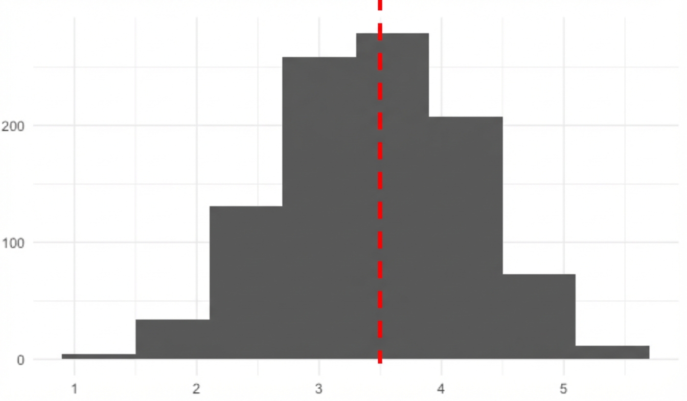
1000 medias muestrales
sample_means <- replicate(1000, sample(die, 5, replace = TRUE) %>% mean())
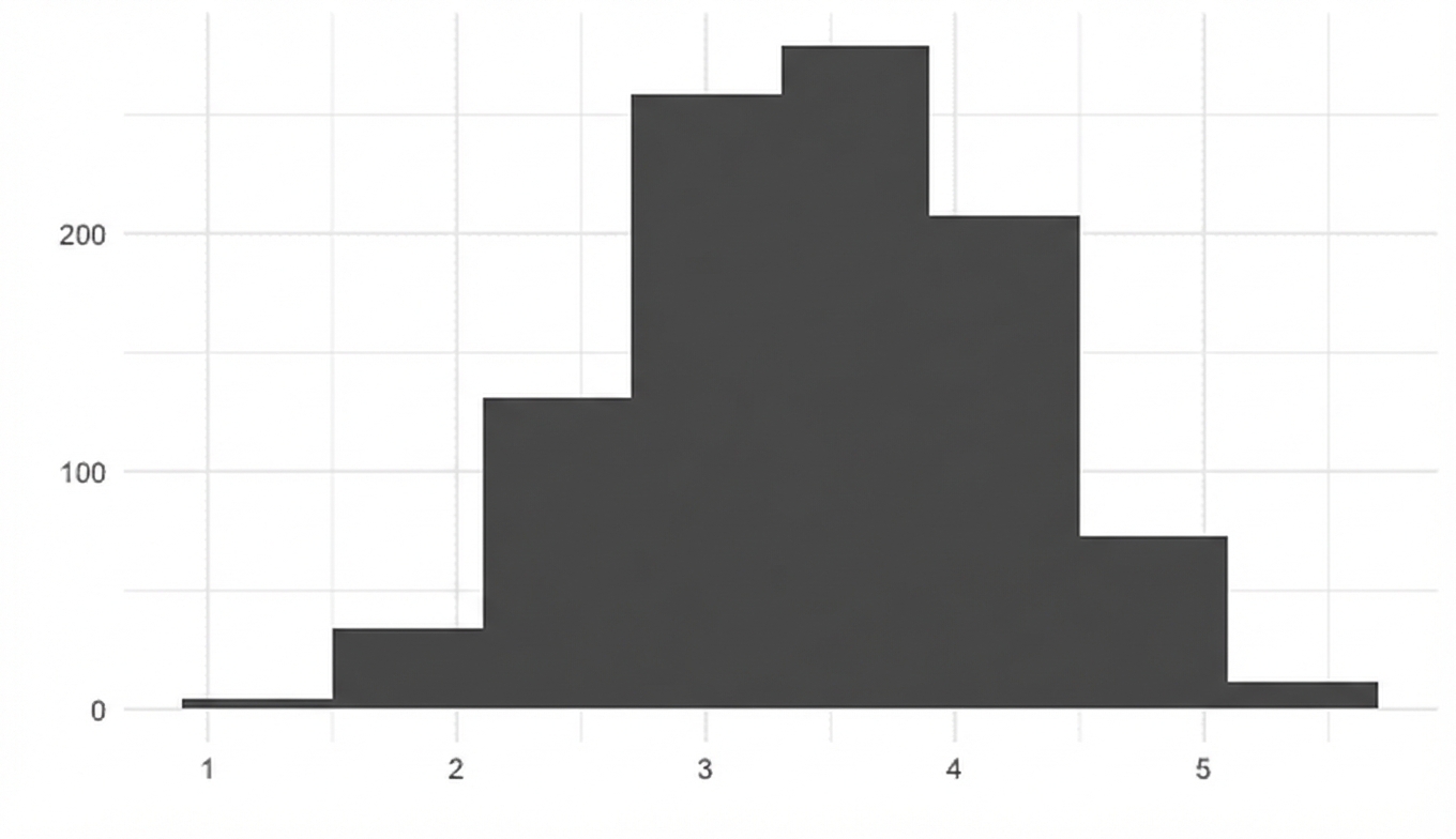
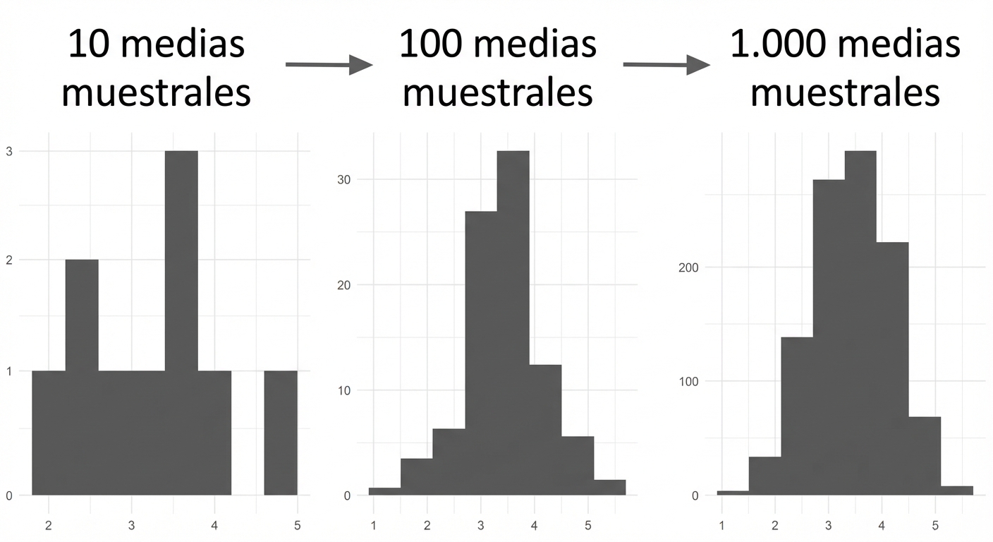
Teorema del límite central
La distribución muestral de una estadística se aproxima más a la distribución normal a medida que aumenta el número de intentos.
- Las muestras deben ser aleatorias e independientes.
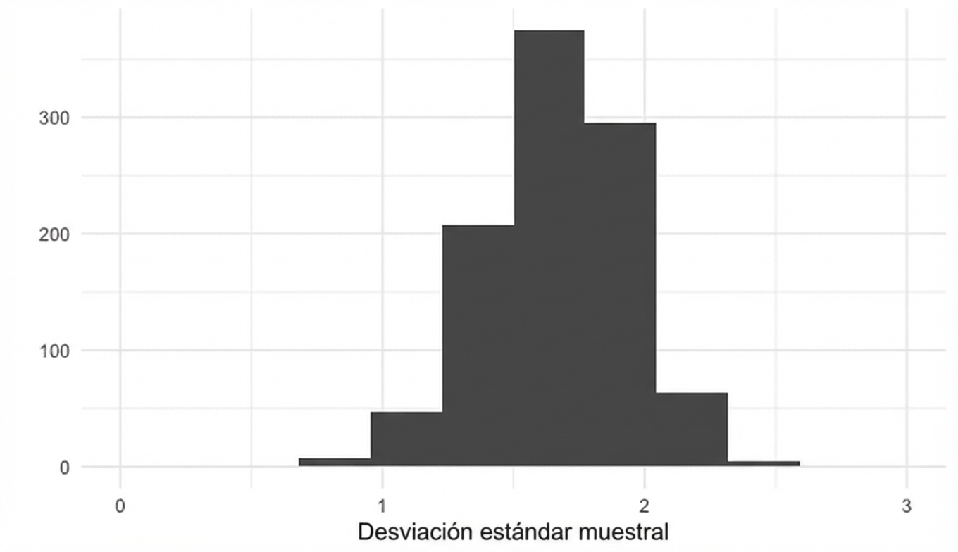
La desviación típica y el TLC
replicate(1000, sample(die, 5, replace = TRUE) %>% sd())
Distribución muestral de la proporción
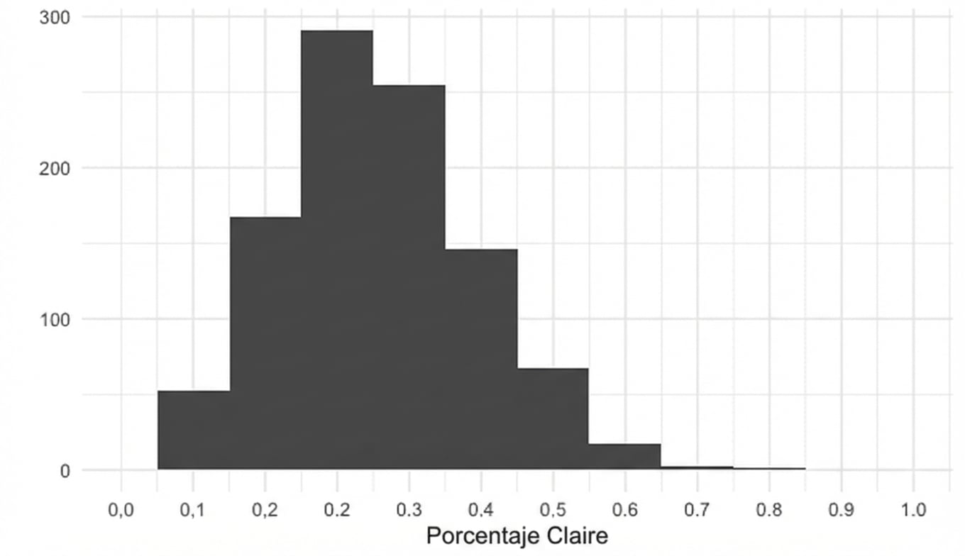
Media de la distribución muestral
- Se estiman más fácilmente las características de grandes poblaciones

