Trabajar con objetos de modelo
Introducción a la regresión con statsmodels en Python

Maarten Van den Broeck
Content Developer at DataCamp
Atributo .params
from statsmodels.formula.api import ols
mdl_mass_vs_length = ols("mass_g ~ length_cm", data = bream).fit()
print(mdl_mass_vs_length.params)
Intercept   -1035.347565
length_cm      54.549981
dtype: float64
Atributo .fittedvalues
Valores ajustados: predicciones sobre el conjunto original
print(mdl_mass_vs_length.fittedvalues)
o, de forma equivalente,
explanatory_data = bream["length_cm"]

print(mdl_mass_vs_length.predict(explanatory_data))
0      230.211993
1      273.851977
2      268.396979
3      399.316934
4      410.226930
    ...
30     873.901768
31     873.901768
32     939.361745
33    1004.821722
34    1037.551710
Length: 35, dtype: float64
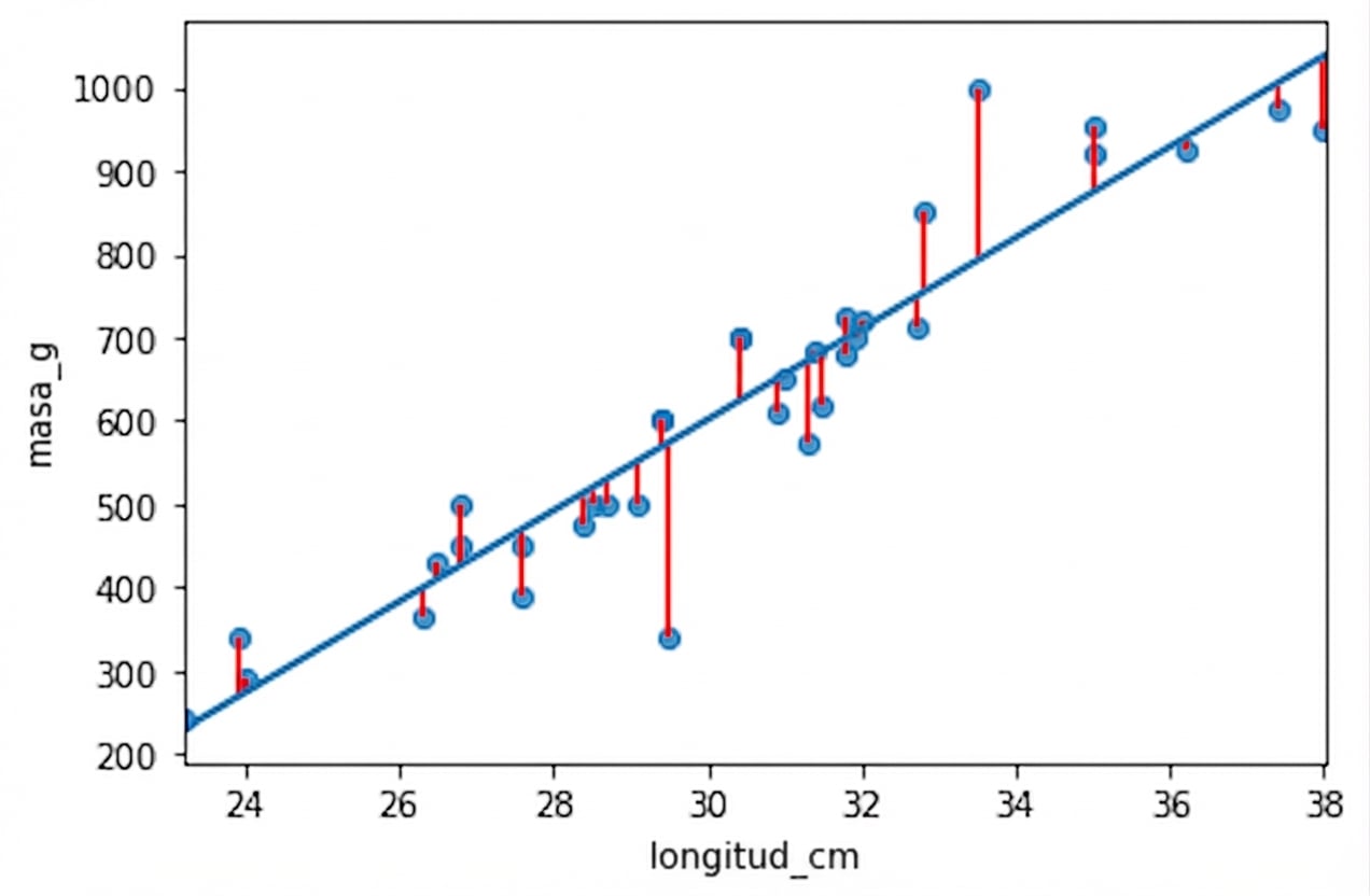
Atributo .resid
Residuos: valores reales menos valores predichos
print(mdl_mass_vs_length.resid)
o, de forma equivalente,
print(bream["mass_g"] - mdl_mass_vs_length.fittedvalues)
0    11.788007
1    16.148023
2    71.603021
3   -36.316934
4    19.773070
   ...
.summary()
mdl_mass_vs_length.summary()
                            OLS Regression Results
==============================================================================
Dep. Variable:                 mass_g   R-squared:                       0.878
Model:                            OLS   Adj. R-squared:                  0.874
Method:                 Least Squares   F-statistic:                     237.6
Date:                Thu, 29 Oct 2020   Prob (F-statistic):           1.22e-16
Time:                        13:23:21   Log-Likelihood:                -199.35
No. Observations:                  35   AIC:                             402.7
Df Residuals:                      33   BIC:                             405.8
Df Model:                           1
Covariance Type:            nonrobust
==============================================================================
                 coef    std err          t      P>|t|      [0.025      0.975]
<-----------------------------------------------------------------------------
Intercept  -1035.3476    107.973     -9.589      0.000   -1255.020    -815.676
length_cm     54.5500      3.539     15.415      0.000      47.350      61.750
==============================================================================
Omnibus:                        7.314   Durbin-Watson:                   1.478
Prob(Omnibus):                  0.026   Jarque-Bera (JB):               10.857
Skew:                          -0.252   Prob(JB):                      0.00439
Kurtosis:                       5.682   Cond. No.                         263.
                            OLS Regression Results
==============================================================================
Dep. Variable:                 mass_g   R-squared:                       0.878
Model:                            OLS   Adj. R-squared:                  0.874
Method:                 Least Squares   F-statistic:                     237.6
Date:                Thu, 29 Oct 2020   Prob (F-statistic):           1.22e-16
Time:                        13:23:21   Log-Likelihood:                -199.35
No. Observations:                  35   AIC:                             402.7
Df Residuals:                      33   BIC:                             405.8
Df Model:                           1
Covariance Type:            nonrobust
                 coef    std err          t      P>|t|      [0.025      0.975]
<-----------------------------------------------------------------------------
Intercept  -1035.3476    107.973     -9.589      0.000   -1255.020    -815.676
length_cm     54.5500      3.539     15.415      0.000      47.350      61.750
==============================================================================
Omnibus:                        7.314   Durbin-Watson:                   1.478
Prob(Omnibus):                  0.026   Jarque-Bera (JB):               10.857
Skew:                          -0.252   Prob(JB):                      0.00439
Kurtosis:                       5.682   Cond. No.                         263.
¡Vamos a practicar!
Introducción a la regresión con statsmodels en Python

